PART D – PREREQUISITE: Earth’s Internal Layering and
Plate Tectonics
Introduction
In PART A - PREREQUISITE, we learned that Earth had differentiated into compositionally distinct layers quite early in its history. In this section, we will learn why that differentiation took place, how we measure the dimensions and character of the internal layers, the extent of dynamic activity within and between those layers, and what the common surface expressions of that activity are.
Layered Planets
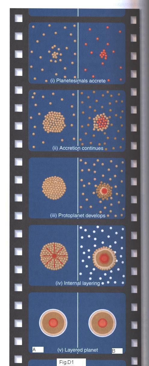
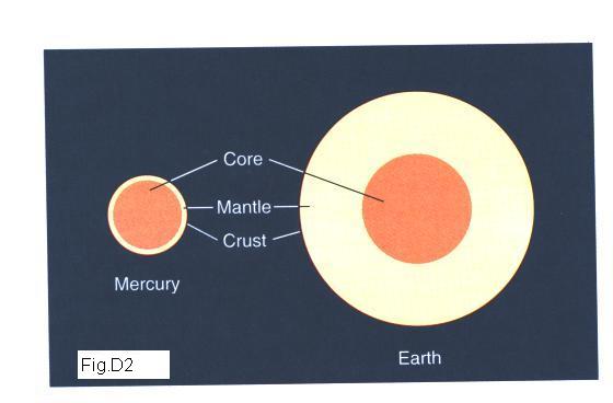
There are two popular models for the formation of planets such as Earth. Both begin, of course, with a process of accretion. The first, called the homogeneous model of planetary accretion (see Fig. D1a) assumes that the material (planetesimals, etc.) which went into the formation of any one planet was more or less similar in composition, thus the resultant planet started out as a homogeneous large body prior to any significant differentiation. As you should guess, the alternate idea is called the inhomogeneous model of accretion (see Fig. D1b). In this model, it is recognized that accretion could go on for quite a long period of time and that differentiation of the accreting bodies may well have occurred prior to being incorporated into Earth. This latter idea is somewhat supported by the evidence we see in meteorites that have come from the bodies of the asteroid belt. In either case, as the growing planet heated from the kinetic energy of impacts and the increasing energy of radioactive decay of unstable isotopes, the result is the same: a layered planet with relatively heavy elements sinking toward the core and relatively light elements being displaced toward the surface. For Earth and Mercury, the layering is nicely illustrated in Figure D2. A detailed ‘pie section’ through Earth appears as Figure D3.
Seismology
How can we possibly know that the boundary between a rigid silicate ‘mantle’ and a liquid metallic ‘core’ lies at 2900 km depth rather than at, say, 2500 km or even 2000 km? In fact, Earth’s internal character was revealed quite by chance while scientists were studying earthquakes. The study of the shock waves of earthquakes is called seismology.
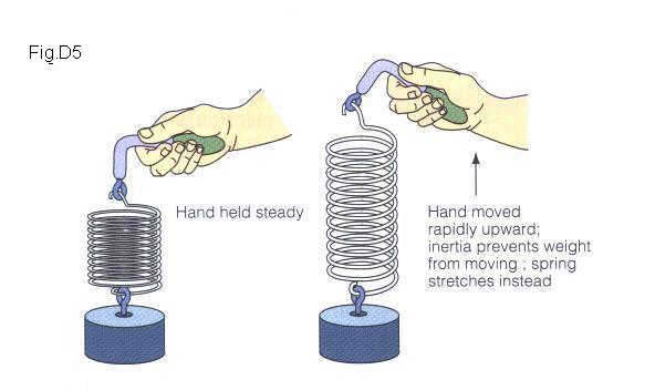
The device used to record the shocks and vibrations caused by earthquakes is called a seismograph (Fig. D4). The ideal way to record the vibrations and motions of the Earth would be to put a seismograph on a stable platform that is not affected by the vibrations of the ground - that is completely isolated from the effects of any earthquake. But, of course, that’s impossible! A seismograph must stand on Earth's vibrating surface, and it will therefore vibrate along with that surface. This means that there is no fixed frame of reference for making measurements. To overcome this problem, most seismographs make use of inertia, the resistance of a large stationary mass to sudden movement. If you suspend a heavy mass, such as a block of iron, from a light spring and suddenly lift the spring, you will notice that because of inertia the block remains almost stationary while the spring stretches (Fig. D5). Using this principal in a seismograph means that the distance between the ground and the mass at the end of the spring may be used to measure vertical (and horizontal) displacement, or motion of the shock wave.
Seismic waves are of two main types: body waves travel outward from the point of origin and have the capacity to travel through Earth. Surface waves, on the other hand, are guided by and restricted to Earth's surface. Body waves are analogous to light and sound waves; surface waves are analogous to ocean waves because they are restricted to a free surface. When we consider earthquakes in detail, we’ll come back to a full discussion of seismic wave characteristics; for now, we will concentrate upon only those properties by which we interpret Earth’s interior layering.
Of the two types of body waves generated by an earthquake shock, the primary (or P) waves are faster. They travel through material as a series of compressions and expansions of molecules (Fig. D6a); they travel rapidly through solids but less rapidly through liquids or gases. Secondary (or S) waves – so-called because they travel more slowly than Primary waves – move through material with a shearing motion (Fig. D6b); as a result, they can only travel through solids (you can’t shear a liquid or gas).
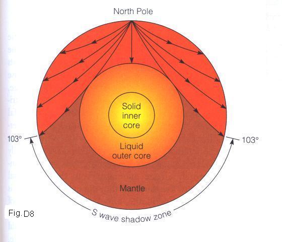
If Earth were perfectly homogeneous, the paths of P-waves and S-waves would spread out from the location of an earthquake in all directions at constant speeds and along straight lines (Fig. D7a). In reality, the speed of seismic waves increases with depth because the density of the materials they travel through increases as the pressure rises within Earth’s deep interior. This causes seismic waves to adopt curved paths, as shown in Figure D7b. In addition to these gradual changes, detailed analysis of the seismic wave paths shows that there are abrupt velocity changes at specific depths within Earth (Fig. D7c); these discontinuities indicate locations of material layer boundaries. In this way, Earth is revealed to be a layered planet consisting of an inner and outer core, a mantle and a crust. For any earthquake of sufficient magnitude that it can be detected at recording stations many thousands of kilometers from its origin, there is always a belt in which no S-waves are ever detected (Fig. D8). Using the geometry of that belt’s location and our knowledge of the rough density of Earth’s mantle, we know that there is a boundary with a major volume of liquid at 2900 km depth (i.e. the outer core).
Many fine-scale features of Earth’s interior have also been defined by interpretation of seismic waves, but we’ll leave that discussion until later.
Taking Earth’s
Temperature
The temperature at Earth’s core is calculated to be 5,500oC (plus or minus 600o); that is based upon the temperature required to melt pure iron metal with 10% impurity (nickel, sulfur, etc.) at 6,370 km depth. Obviously, there’s no possibility of any direct measurement. Out as far as the core-mantle boundary, the temperature should be only 4000oC (again, based upon the minimum melting of core material for the pressure represented by 2900 km depth). Through the mantle, which we know to be composed of dense silicates and oxides, we watch the variations in seismic wave velocity to tell us about temperature variations. We will look at some of those variations later in the course. Right now, we can graph Earth’s internal temperature, in general terms, in Figure D9.
At 5,500oC, Earth’s core is nearly the same as our Sun’s surface. How did this planet get so hot? In fact, while Earth’s very earliest days were pretty cool, the transfer of kinetic energy from impacts, the enormous energy yielded by radioactivity, and the heat produced by transfer of matter from core to crust to produce layering all soon produced a really hot world. The impact of a Mars-size planet that eventually resulted in our Moon certainly contributed enormous energy to Earth, and resulted in a completely molten planet. One painter suggests Earth’s surface looked similar to Figure D10. Ever since those early days, Earth’s interior has been cooling, although the rate of cooling is very slow.
Convection, Mantle
Plumes, a Cooling Earth, and Plate Tectonics
Cooling Models
What is a possible mechanism by which Earth’s interior might cool? Heat conduction through a solid is familiar to us all, perhaps through something as simple as noting that the handle of a metal spoon heats as you stir hot coffee! But most rocks are relatively poor heat conductors, so conduction is not likely to be the major cooling mechanism for Earth.
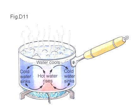
Early consideration of the cooling problem led to the simple convection model, as illustrated by the currents developed in a pan of water over a heat source (Fig. D11). In the pan shown, water rises and falls according to a very specific pattern. As water molecules are heated, they expand slightly (the distances between the atoms of oxygen and hydrogen increase slightly), resulting in molecules that are just a bit less dense, so they rise. At the top of the pan, the water molecules cool slightly, become just a bit more dense, and thus fall toward the bottom of the pan. This cyclical pattern of motion is called convection.
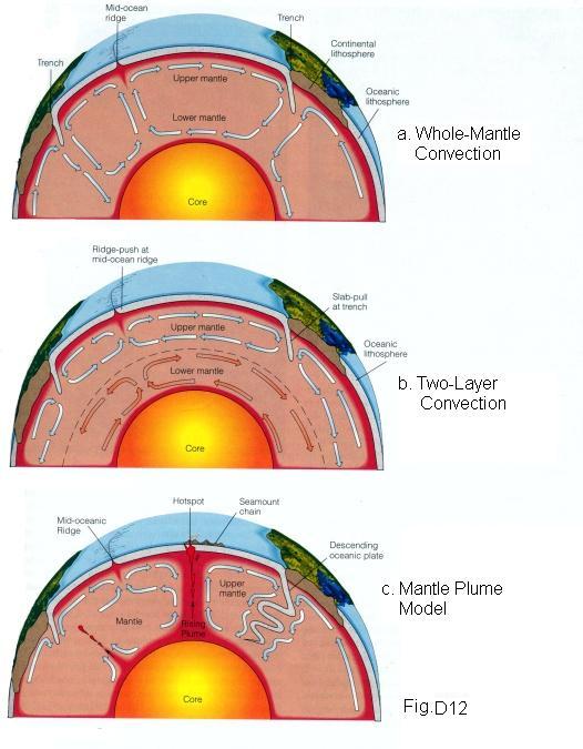
Convection is obviously an excellent process to move heat from one region of a medium to another, thus it’s natural to expect it to be considered as a possible mechanism within Earth. Of course, no one is suggesting that Earth’s mantle is as fluid as water, but suppose it might act as a moderately malleable plastic? With that assumption firmly in mind, scientists proposed the ‘whole-mantle convection model’ as illustrated in Figure D12a. Convection cells must operate in pairs (they’d cancel each other out if the vertical component motions were in opposite directions), thus a neat geometric sequence was envisaged to operate within Earth. Scientists remembered, however, that seismic wave patterns had indicated the presence of a major horizon part way down in the mantle that marked a significant variation in physical properties of mantle material; this is the boundary between apparently ‘soft’ asthenosphere (or upper mantle) and much more rigid mesosphere (or lower mantle). It was thought that there was some difficulty in material ‘communicating’ across that boundary, so the ‘two-layer convection model’ was born (Fig. D12b). In fact, it has probably caused more problems than it’s solved, so a new and better model is now in place.
The new model, quite rightly, takes note of the fact that
there commonly are sites on Earth’s surface considerably hotter than can
readily be accounted for by any convection theory. Also, technology has
advanced dramatically in the last few years, and we are now able to
significantly refine our interpretation of seismic and heat flow signals. The
new model is called the ‘mantle plume
model’, and it’s illustrated in Figure D12c. Note that
convection still plays a significant role, but by far the dominant features are
columns of heat, called plumes, the rise straight through the mantle from the
core-mantle boundary. Toward Earth’s surface, these heat plumes produce melting
of mantle material resulting in long-term volcanism (such as at
Plate Tectonics
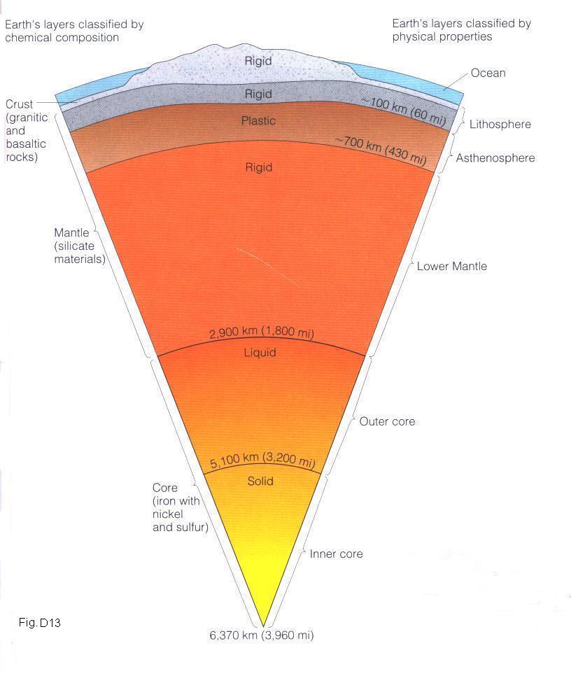
With such motions as illustrated above taking place in
Earth’s mantle, the cool, brittle outer part of Earth, called the lithosphere
(Fig. D13) is
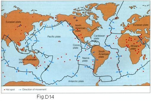
placed under considerable stress. That motion has, in
fact, torn Earth’s brittle lithosphere into segments we call plates (Fig. D14); there are 7
large plates and several smaller ones. For ease of reference, we apply names to
those segments or plates. For example, Halifax and Vancouver (east-west), and
If we looked closely at the plate boundaries, we’d see that
just west of
There is a term that refers to all this activity: plate tectonics. Plate tectonics is called the unifying concept of geology because it provides a coherent model of the outer part of Earth and how it works. There are only three ways segments or plates of a globe can interact (Fig. D16) and, therefore, three types of boundaries: divergent, convergent, and transform. Each of the three boundaries is produced by different stresses:
Because many details
of plate tectonics are interwoven with our scenarios of catastrophic events, we
will return to this topic in the lecture content of 240A. Please resume the
regular lecture sequence.