Click here to return to course outline.
A chemical element is identified by its Atomic Number, Z, which defines both the number of protons (Proton Number) in the nucleus and the number of electrons in the neutral atom. The number of neutrons the atom contains is referred to as the Neutron Number, and the sum of the Proton and Neutron Numbers is the Atomic Mass Number. In the following notation for iron:
57
FE
26
the value 57 refers to the atomic mass number
of iron, and the value 26 to the atomic or proton
number. Atoms that can be uniquely identified in terms of their
proton numbers and atomic mass numbers are collectively called nuclides.
Nuclides that have the same atomic number but different neutron numbers
are called isotopes of an element.
Nuclides with the same neutron number but different mass number are called
isotones,
whereas those with different proton or neutron numbers and the same mass
number are called isobars. There are
81 stable elements comprising 264 stable nuclides.
Unstable nuclides
are calle radionuclides. Neutron rich
radionuclides decay by ejecting an electron when an neutron is converted
to a proton, e.g. 87Rb (Z=37) to 87Sr (Z=38), whereas proton-rich radionuclides
tend to convert to isotopes of lower atomic number by capturing an electron,
e.g. 40K (Z=19) to 40Ar (Z=18). These reactions are isobaric. Decay may
also take place by the emission of a Helium atom or alpha-particle composed
of 2 protons and 2 neutrons, e.g. 147Sm to 143Nd, whereby the atomic mass
number decreases by 4 mass units, and the proton and neutron numbers by
2 units.
Almost all of the elements exist in several isotopic forms, but
only about 250 elements are stable and exist in measurable quantities,
and only 51 of the known radioactive isotopes exist in nature.
Elements of atomic mass number
less than 20 (e.g. H, O, N, S, C) exhibit variations in isotopic composition
that are detectable by modern means of measurement, whereas most elements
with mass number greater than 20 tend to show constant isotopic composition.
The exceptions, K, Ar, Rb, Sr, Sm, Nd, Rh, Os, and U, Th, and Pb, vary
in composition because they include varying proportions of the parent and
daughter products of radioactive disintegration.
The measurement of the relative
concentration of isotopes in rocks is extremely useful as a means:
1) to establish the tectonic environment of formation of rocks;
2) to determine the age of rocks;
3) to estimate the physical conditions of the hydrosphere and atmosphere
at the time of
sedimentary rock deposition; i.e. to act as chemostratigraphic markers.
4) to estimate the nature of the source rocks of hydrothermal mineral deposits.
References: Faure, G., Principles
and Applications of Geochemistry, 2nd ed, Prentice Hall.
Brownlow, A.H., Geochemistry, 2nd ed, Prentice Hall.
Allegre, C-J., and Michard, G., Introduction to Geochemistry, Reidel.
Isotopic studies in Paleontology, Journal of the Geological Society, v.
154, p. 293-356
The Stable Light Isotopes
The non-radioactive light
elements oxygen, carbon and sulphur, which are commonly referred to as
Stable Isotopes, are valuable in understanding geological processes because
they may undergo fractionation when the phase in which they occur changes
state (e.g. oxygen in water changing from liquid
to gas or solid), or participates in a chemical reaction involving a change
of state (e.g. sulphate versus sulphide in the case of sulphur). Consequently,
the oxygen isotopic composition of sea water differs from that of both
polar ice, atmospheric water vapour, or rain water, where the seas and
polar ice can be considered to represent independent end-member water reservoirs
in quasi-equilibrium with each other. The Raleigh
fractionation of the oxygen isotopes takes
place during the sequential removal of rain water from atmospheric
vapour as the vapour is transferred from its place of origin (evaporation)
in the tropics towards the polar ice reservoir. Note that if there were
no polar ice-reservoir most of the atmospheric water vapour would be returned
to the oceans, and all things else being equal, the oxygen isotopic composition
of the oceans would be constant.
Similarly, carbon in sea water is fractionated as a result of biogenic
activity, carbon-based life forms favouring the concentration of 12C over
13C. However, as in the case of water vapour, once the 'bugs' die their
carbon would be returned to the oceans, which would therefore exhibit only
a secular variation in isotopic composition related to variations in the
rate of biogenic activity. On the other hand, if a significant fraction
of the 'deceased' were to be buried during sedimentation, the sedimentary
rocks would constitute a separate carbon reservoir, and the isotopic composition
of sea water would then reflect the relative rates of biogenic activity,
sedimentation, and the erosion of carbon rock reservoirs. Fractionation
would be a maximum at high rates of biogenic activity and sedimentation,
and low rates of erosion.
In
the case of sulphur, the isotopic fractionation takes place as a result
of the bacteria-mediated progressive (Raleigh)
conversion of ocean water sulphate to 32S enriched hydrogen sulphide, and
the removal of the latter into a separate rock reservoir as pyrite. Note
again that if the hydrogen sulphide is not separated out of solution, or
if all the sulphate were to converted to sulphide, the isotopic composition
of the sea water would not change.
Oxygen
Average abundance ratio 18O/16O ratio = 0.2/99.762 = 0.0020048 = 1/498.81
Isotopes of oxygen are fractionated when they pass from the hydrosphere to the atmosphere such that, for example, oxygen becomes enriched in the light oxygen isotope 16O relative to the heavy oxygen isotope 18O. Numerically, the variation (known as d18O) is expressed in terms of the deviation of the ratio of 18O to 16O in the sample of material being analyzed from the mean value of 18O/16O in seawater (SMOW, standing for Standard Mean Ocean Water), viz,
d18O = (18O/16Osample - 18O/16OSMOW)/18O/16OSMOW * 10^3 °/°°
(Note 1: 18O/16O ratio of SMOW is 0.0020052; if
the sample is enriched in light oxygen 16O such that 18O/16O
is less than this value, the d18O
value will be negative )
(Note 2: the oxygen isotope composition of carbonates is commonly expressed
relative to a carbonate standard known as PDB (Peedee belemnite), where
d18O
(SMOW) = 1.03086 d18O (PDB) + 30.86.; the d18O
value of carbonates is usually much greater than that of SMOW).
(Note 3: the variation in relative concentration of Hydrogen and Deuterium
tends to mimic that of 18O and 16O, repectively, and the variation relative
to SMOW in this case is represented as dD.
Mantle materials have d18O
values of about +5 to +6, whereas rain water may have values as low as
-50 at the South Pole. One might anticipate that atmospheric oxygen (O2)
would also be relatively light. However, it is highly positive as a result
of fractionation related to biological respiration (Dole effect) - biogenic
materials always tend to concentrate the light isotope. Note that the isotopic
composition of oxygen produced by photosynthesis is related to the isotopic
composition of the hydrous enviroment.
Oxygen isotope variation in rocks.
Because rain water fractionates heavy oxygen out of atmospheric moisture (16O increases and 18O/16O decreases), the moisture therefore becomes progressively enriched in light oxygen as it moves from warm equatorial latitudes towards the cold polar regions. Polar ice therefore constitutes a reservoir of 16O enriched water separate from sea water. The isotopic composition of the latter is therefore controlled by the magnitude of the polar ice regions. Melting the polar ice caps would decrease the d18O value of sea water.
Oxygen isotope variation in precipitated waters.
Clay minerals formed during
weathering may have positive d18O values, varying
from +10 at high latitudes to +30 at low latitudes (nearer the equator),
and carbonates here may have values as high as 34. (see Faure p. 353 for
the values for marine shales.)
The measurement of d18O
values provides a relatively simple means of 'fingerprinting' fluids involved
in hydrothermal mineralization, hot spring formation, and diagenesis. Note
that in the case of hot springs (see following diagram) ground water oxygen
'gets heavier' (d18O is less negative) as it
equilibriates with the rock through which it passes
.
Oxygen
isotope variation in thermal waters.
In a less simple manner,
the penetration of sea water through oceanic basalt causes the d18O
of the basalt to initially increase and then to decrease once the temperature
reaches that of the upper greenschist facies.
While the removal
of light water to form polar ice causes the
d18O
of sea water to
increase,
the precipitation of carbonate with a positive d18O
value causes a
decrease in the d18O
value of seawater. Furthermore, a decrease in sea water temperature causes
an increase in d18O of precipitated carbonate,
thereby tending to accentuate the decrease
in the d18O value of seawater. With
a fall in temperature therefore, carbonate precipitation will tend to counterbalance
any increase of the d18O of the sea water through
the removal of water in the form of polar ice.On
the other hand a decrease in average oceanic temperature will
increase
the solubility of carbonate, thereby minimizing the effect of carbonate
precipitation. To relativize the effect of polar ice and carbonate precipitation,
it is necessary therefore to analyze the shells of both surface living
planktonic foraminifera and the shells of deep-dwelling benthic species
living at relatively constant temperature.
Advanced Reading: Huber, BT., MacLeod, K.G., and Wing, S.L., 1999. Warm Climates in Earth History. Cambridge University Press, 462p., US$115; review by Bednarski, J.M., Geoscience Canada, v. 27, 4, 189-191.
Carbon
Recommended background reading: Berner, R.A., 1999, A new look at the long-term carbon cycle. GSA Today, v. 9, no. 11, p. 1-6.
Average 13C/12C ratio = 1.1/98.9
= 0.0111223 = 1/89.9091
In calculating the d13C
values of organic material, the carbon standard used is the limestone of
a fossil belemnite from the Pee Dee Formation (PDB) of North Carolina.
Living
organisms preferentially concentrates 12C relative to 13C, and
the d13C (PDB) isotope values of plants that
use the C3 metabolic process ranges from -23 to -34 per mil, whereas those
(corn, tropical plants) that use the C4 process ranges from -6 to -23 (Beerling,
1997, p.303). (The advent of C4 vegetation took place in the Miocene.)
CO2
removed from soils by plant respiration is also enriched
in 12C and therefore isotopically light (c. -27 per mil)
in
comparison with normal atmospheric CO2 (-6 per mil). Because
of the preferential removal of 12C by plant respiration,
palaeosol
carbonates (carbonates in soils) will therefore evolve in the
direction of higher (less negative)
d13C values.
On the other hand,
fossil fuels are
strongly enriched in 12C relative to 13C , that is they have lower or more
negative d13C values reflective of their
organic derivation.
Bicarbonate
formed
from atmospheric CO2 (d13C - -6 per mil.
PDB) entering solution:
CO2 + H2O = HCO3- +H
+
is enriched in 13C, and when CaCO3 precipitates from bicarbonate solution:
Ca(HCO3)2 = CaCO3 +
CO2 + H2O
it is further enriched in this
isotope. The d13C (PDB) of Phanerozoic marine
carbonate rocks therefore tends towards a value of 0.
[Note that precipitation
of CaCO3 and release of CO2 to the atmosphere is favoured by rising temperatures.
The increase in CO2 can only be mitigated by an increase in weathering
reactions, e.g.
Primary material
Weathered material
CaAl2Si2O8 (Anorthite) + 3H2O
+ 2CO2 = Al2Si2O5(OH)4
(Clay) + Ca(HCO3)2]
Secular changes in the isotopic
composition of the aquatic primary producers are related to the concentration
of CO2 in the atmosphere, where the isotope fractionation
associated with the photosynthetic fixation of carbon is proportional to
the log value of the concentration of dissolved CO2. The d13C
of organic carbon can therefore be
used to provide a likely record of the abundance of atmospheric CO2 (Beerling,
p. 304), and from the limestone organic carbon record it would seem that
atmospheric concentration of CO2 was high at the end of the Cretaceous
(1000 ppm) and has decreased (< 400 ppm) ever since that time (Beerling
p. 305). In contrast the 87Sr/86Sr of sea water has consistently increased
since the end of the Cretaceous, implying that weathering/erosion of continental
crust has been increasingly more effective.
The value of 13C/12C relative
to that of a standard limestone (Peedee belemnite), d13C,
is controlled 1) by the level of biotic activity in the oceans (which is
itself controlled by the availability of nutrients); and 2) the rate of
removal of the organic carbon (and of nutrients) by burial relative to
its return to the oceans by weathering, solution, and the precipitation
of carbonates. High rates of biotic activity and of carbon burial, that
is high rates of removal of 12C, will cause sea water to develop a relatively
high d13C value (e.g. +8 per mil). For this
reason a d13C minimum (more 12C = decrease in
the ratio 13C/12C = negative d13C excursion)
follows some sudden extinction events because the reduced biotic activity
diminishes removal of 12C, whereas a relatively large amount of 12C represented
by the deceased bugs is dissolved back into the seawater.
High d13C
values may therefore reflect high levels of biotic activity in well developed
optimum-sized shelf seas receiving a strong flux of dissolved nutrients
(phosphorus), as well as an abundant supply of clastic sediment to rapidly
bury the biogenic carbon being produced. Polar ice caps would generate
active deep-water cold water currents that would also be effective in supplying
nutrients to the shelf, and the magnitude of the ice caps would control
the degree of transgression or regression of the seas onto the continents.
Should conditions move towards a 'snowball' Earth,
the shelves and associated biotic activity might be forced into a sharp
recession, and d13C values would markedly decrease.
On the other hand, an increase in oceanic tectonic activity might cause
excessive flooding of the continents (high flux of greenhouse CO2 leading
to the melting of the ice caps), which in turn would turn off the supply
of nutrients and of sediment. The flux of mantle derived CO2 with d13C
of about -7 /mil would also tend to decrease the d13C
of ocean water.
Examples
in the Geological Record
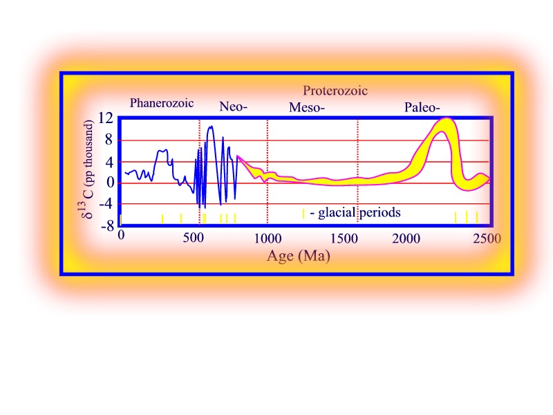
The Paleo-Proterozoic included
a period of negative
d13C excursions perhaps
coincident with the Huronian Gowganda glaciation, followed by three positive
excursions in the interval 2.43 to 1.93 Ga (Geology 1998, p. 875). In contrast,
d13C
for the Meso-Proterozic until 1 Ga ago remained relatively constant with
values of about 0. During the Neo-Proterozoic,
d13C
values once again increased to values greater than 10 (significant increase
in biotic activity) punctuated by high-amplitude negative excursions coincident
with periods of 'snowball' Earth glaciations; implying very sudden terminations
of biotic activity.
Secular variation in d13C since the Archean
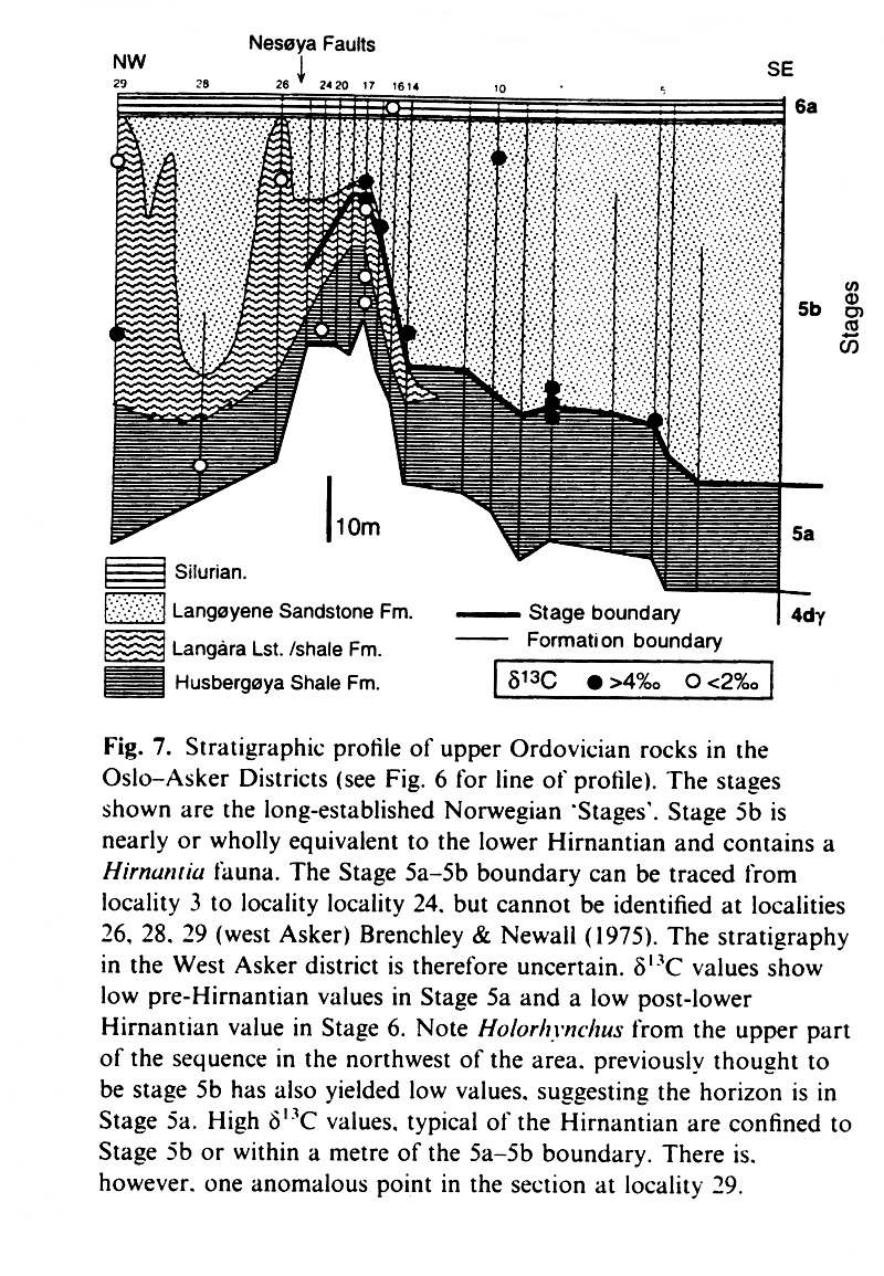
The late Ordovician (Hirnantian)
faunal extinction was accompanied by the onset in growth of ice caps, a
fall in sea level of a 100 metres, and an increase of d13C
from 0 to +6 (all values per mil PDB) of sea water (there might be an increase
in burial rates and decrease in erosion and therefore of the rate of transfer
of 12C to the oceans, as well as an overall increase in biotic activity
due to increased nutrient supply from the polar regions to the shelves),
as well as of
d18O from -4.5 to -1.5 (an excursion
to less -ve values reflects the transfer of more light 16O to the icecaps).
Stable
isotope curves for brachiopod compositions variation during the late Orodovician
Hirnantian stage (Brenchley et al. 1997) - hirnantian1.jpg
Stratigraphic
profile of Upper Ordovician rocks of the Oslo (Norway) region (Brenchley
et al, 1997) - hirnantian2.jpg
Similar positive excursions
(-1 to 7.5 d 13C), have been recognized at three
levels in the Silurian (BGSA 1999, p. 1499) and correlated with sea-level
lowstands, and the Carboniferous glaciation was marked by a positive
d13C
excursion to +6 per mil.
A decrease in d13C
of 3 per mil during the Artinskian and Kungarian of the early Permian,
and a general decrease (more negative) change at the Permian - Triassic
boundary (250 Ma), was commensurate with a relative decrease in 13C in
the oceans and atmosphere, that is, an increase in 12C. By 250 Ma the supercontinent
Pangaea was complete, but subject to uplift around its margins due to the
tectonic compressive stress of collision. As a result, the vast peat reserves
in the coal-bearing foreland basins of Pangaea were oxidized leading to
a massive flux of CO2 with low d13C values into
the oceans; plunging d13C values once again
to about 0 per mil.
At the Cretaceous-Tertiary
boundary, reduced light levels, supposedly due to meteorite impact, inhibited
phytoplankton, and then the zooplankton feeding on the phytoplankton, and
other life forms feeding on the phytoplankton, causing a negative 13C excursion
- that is more 12C was returned to the oceans than was removed by biotic
activity.
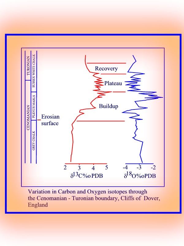
At the Cenomanian - Turonian
boundary large quantities of organic carbon were produced causing a marked
+ve d13C excursion for sea water. The increase
in biotic activity was however accompanied by an increased burial rate
of the carbon, thus causing nutrients to be removed from the system (i.e.
no food). This caused a decline in photic zone coccolith production and
carbonate accumulation rates, which in turn starved the zoooplankton and
caused their selective extinction. There was therefore a return to lower
d
13C values (negative
d13C excursion; more 12C
was dissolved into the oceans than was removed by the biotic activity).
Higher temperatures at this time also reduced coccolith (carbonate) productivity.
Isotope curves through the Cenomanian-Turonian boundary.
Rocks that contain buried carbon are characterized by a -ve d13C values, and the carbonate in quartz veins containing Au flushed from sedimentary rocks invariably exhibits -ve d13C values (e.g. -20 per mil).
In the case of 14C equilibrium:
14C in the descending flux = 14C in ascending flux
(W.Cs + B).Rs = W.Cd.Rs
and
W.Cd.Rs = W.Cd.Rd + Vd.Cd.Rd.l
where Rd < Rs because
of the loss by radioactive disintegation of 14C in the the total volume
Vd.
Therefore,
WRd + Vd.Rd.l = W.Rs
W.(Rs - Rd) = Vd.Rd.l
W/Vd = Rd.l /(Rs - Rd)
and residence time = (total
carbon in deep zone/carbon descending /year from upper zone to lower zone,
= Vd.Cd/W.Cd = Vd./W = (Rs - Rd)/(Rs.l )
If l
= 1.25 x 10⁻⁴ yr-1), the residence time is about 100 years.
Study of the variation of
14C in the worlds oceans has lead to the distinction of 6 large oceanic
reservoirs.
Average abundance 34S/ 32S = 4.21/95.02= 0.0443065 = 1/22.570071
32S/34S in various rock types.
Sulphur fractionation is
evident in the relative variation of the sulphur isotopes 32S and 34S,
usually expressed as a d value relative to a
standard 32S/34S ratio of 22.225, the value of the Canyon Diablo Troilite
meteorite and close to that of most mantle derived mafic rocks.
(Note 4: in some conventions
the ratio of isotopes are given as the ratio of the more abundant isotope
to the less abundant isotope, whereas the calculation of d
values uses the ratios of heavier to lighter isotopes. Because 32S is more
abundant than 34S, sulphur isotope ratios in the above graph are presented
as 32S/34S and have values greater than unity. Consequently, positive d34S
values in the graph plot to the left of 0, and negative values to the right.)
Sulphur isotopes are fractionated because the heavier isotope is preferentially
taken up by the compound in which sulphur is most strongly bonded, sulphate
as distinct from sulphide in the case of 34S. The d34S
values of sulphates in sea and fresh water range from +4 to +30, with a
value of +20 more typical of sea water, whereas the sulphides associated
with mineral deposits range from +7 to -7 in igneous rocks and +50 to -45
in sedimentary rocks.
In recent marine sediments
it has been observed (Kaplan 1983) that bacterial
reduction of sulphate causes the dissolved H2S in pore water in the sediment
to become enriched in 32S and the sulphate to become enriched in 34S.
If the hydrogen sulphide escapes out of the pore water, the dissolved sulphate
and total sulphur in the downward circulating pore water will consequently
decrease, and the dissolved sulphate will be progressively enriched in
34S (Raleigh distillation). If the pore water is returned to the oceans,
the latter would become enriched in 34S. H2S produced from this sulphate
by bacterial reduction will then also be relatively enriched in 32S but
progressively less than that formed earlier. If the H2S is fixed
as pyrite, the latter will take on the enriched 32S isotopic characteristics
of the H2S (negative d values) from which it
was formed. On the other hand pyrite formed directly from the 34S enriched
sulphate will exhibit positive d values.
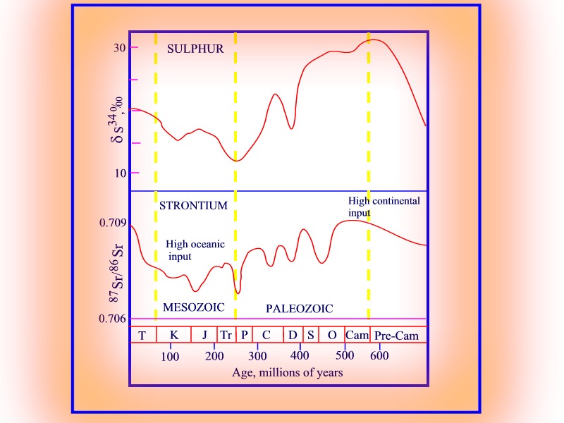
The isotope evolution of
S in the oceans is very similar to that of Sr. Both show high d
values during the late Proterozoic - Cambrian and the Present, and minimum
values during the Mesozoic. The isotopic character of the Sulphur contributed
by the continents to the oceans will however depend upon the relative contributions
of weathered sulphates (evaporites) and sulphides (igneous and sedimentary
rocks). The isotopic character of sea water will also be controlled by
the relative rate of formation of evaporite deposits, the effectiveness
of bacterial activity in reducing sulphate taken from the oceans, the rate
of introduction of cold oxygenated waters from the polar regions (sulphate
production versus biotic activity), and the rate of removal of sulphide
by reactive volcanic Fe.
What would be the optimal
conditions for high 32S/34S levels (low d values)
in ocean water:
1) high rate of formation of evaporite and high
erosion rates of d-negative sulphidic sediments;
2) low volcanic activity = low Fe = low sulphide removal; 3) high oxygenated
water = conversion of insoluble pyrite to soluble sulphate without sulphur
fractionation; 4) low bacterial rate of reduction of sulphate if sulphate
is returned to the oceans.
Variation in Sulphur and Strontium isotopes in seawater since the late Proterozoic.
C/S ratios
The C/S ratio of normal marine sediments (deposited beneath oxygenated waters) is c. 2.0 in Late Paleozoic and younger rocks, but as low as 0.5 in older Paleozoic sediments. The difference is attributed to the advent of land plants in the Late Silurian and the fact that terrestrial organic matter is less easily metabolized (less labile) than marine organic matter. The presence of less reactive plant material in the sediment therefore increases its C/S ratio. However, some Cambrian sediments have ratios as high as 1.4, suggesting that values as low as 0.5 may reflect the increased presence of reactive Fe in the form of volcanic glass that would trap the bacterial formed hydrogen sulphide as pyrite. That is, the lower C/S ratio is due to increased sulphur content rather than decreased carbon content.
The C-S-O cycle
Bacteria mediated:
2CH2O + H2SO4 = 2CO2 + H2S
+ 2H2O (removal of C and S from the oceans to the atmosphere)
Photosynthesis:
2CO2 +2H2O = 2CH2O + 2O2
(conversion of CO2 to O2, and addition of C to the oceans)
Oxydation:
H2S + 2O2 = H2SO4 (return
of S and O to the oceans from the atmosphere).
These three equations balance out, and are rate rather than thermodynamically controlled. The rate relationship can be perturbed by, for example, the addition of volcanic ferrous iron, or the rate of burial of CH2O, or erosion of sulphate deposits, or removal of CO2 as carbonate from the oceans.
Radioactive elements are
useful for two reasons:
1) they allow the determination
of the age of rocks and minerals;
2) they can be used to 'fingerprint'
the primary source of rock and mineral material.
The main isotopic systems are those of K and Ar, Rb and Sr, Sm and Nd, U or Th and Pb, and Rh and Os, where in each case the first element of the pair is the parent isotope and the second element the daughter isotope. In the case of the 87Rb-87Sr nuclide pair, 87Rb, whose proton number is 37 and whose neutron number is 50, changes to 87Sr with a proton number of 38 and a neutron number of 49. In this case the change involves the conversion of one neutron to one proton plus one Beta particle and an antineutrino. On the other hand 147Sm (proton number 62) changes to 143Nd (proton number 60) by the loss of a 4He atom or alpha particle (2 protons and 2 neutrons), whereas the conversion of U to Pb takes place via a series of spontaneous fission reactions.
The Law of Radioactivity
In the following description
we will use the example of Rb/Sr, although the same calculation applies
to any of the parent-daughter pairs mentioned above. The law of radioactivity
states that the rate of decay of the parent element at any time during
its decay is proportional to the number of atoms of the parent present
at that time. A plot of 87Rb as ordinate against Time as abscissa will
therefore define a curve which will be negative and whose slope will decrease
with the passage of time. The equation of the curve will be: -dRb/dt =
l.Rb
(where l is the decay constant) and therefore:
-dRb/Rb = l.dt
Integrating dRb and dt from time t0 to time tn (now):]
-(lnRbtn-lnRbt0) = l d
t and ln[Rbt0/Rbtn] = l.dt and Rbt0 / Rbtn =
e^l.dt ;
and
Rbt0 = Rbtn e^l.dt
This relationship allows us to
calculate the 87Rb content of a rock or mineral at any time in the past
from its present day value.
Since the amount of daughter
product, 87Sr = 87Rbt0 - 87Rbtn and the initial
amount of 87Sr in the rock at time t0 = Sri
then the total amount of 87Sr = 87SrT = 87Sri
+ (87Rbt0 - 87Rbtn) = 87Sri + (87Rbtn e^l.dt
- 87Rbtn)
= 87Sri + 87Rbtn (e^l.dt
- 1)
Since SrT and Rbtn can be
measured, and delta is a constant, the age of the rock, delta t, can be
calculated if we also know the value of Sr0, the initial amount of
87Sr in the rock. This however we cannot know, and even if we were to construct
a second equation using data from a second specimen with a different 87Rb
and Total 87Sr, we still cannot assume that 87Sri
will be same in both specimens. The problem can be solved, however, if
we assume that the relative proportions of the various Sr isotopes in all
coeval and consanguinous samples is constant. In this case the ratio of
87Sr to the stable Sr isotope 86Sr will be the same in all specimens, even
if the actual amount of 87Sr is different. The above equation can then
be converted to the form:
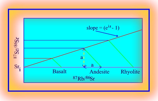
(87Sr/86Sr)T = (87Sr/86Sr)i + 87Rbtn/86Sr
(e^l.dt - 1))
Two or more samples of the
rock with different (87Sr/86Sr)T and 87Rbtn/86Sr values would then allow
the writing of a set of simultaneous equations from which delta t can be
calculated.
The above equation has the form of a straight line, Y = AX + B, where (87Sr/86Sr)i, commonly known as the 87Sr/86Sr initial ratio (Sri), is the intercept, and (e^l.dt - 1) the slope of the line. Consequently, the values of these parameters can be determined by graphing 87SrT/86Sr against 87Rbtn/86Sr. Such a graph (above) is known as a Nicolaysen graph, and is the preferred method of representing isotopic data in the calculation of rock and mineral ages. Both Rb and Sr behave as relatively incompatible elements in basaltic liquids. Consequently, radiogenic Sr in the basaltic crust will grow at a faster rate than the primary mantle (Bulk Earth), which will itself produce radiogenic Sr at a faster rate than the depleted mantle. If at any time subsequent to the formation of the basalt, any or all of these independent reservoirs again undergoes melting, the Sri of the melts will reflect that of the reservoir from which they are derived. Melts derived from depleted mantle will have lower Sri values than melts derived from undepleted mantle, which will have Sri values lower than melts derived from the basaltic crust.
It is important to note that
the Sri values of the melts from the reservoirs is independent of the mineralogy
of the reservoir or the amount of melt produced, because the Sr isotopes
are not fractionated by physical processes involving solids and liquids
in the crust or mantle. The Sri values are determined by the initial Rb
contents of the reservoirs following melting, and the time since the melting
event. Because MORB basalts have low Sri we know that the mantle from which
oceanic basalts are derived is depleted in Rb as well as in the associated
elements K and Ba. On the other hand WP basalts have relatively high Sri
values, indicating that the mantle source of WPB's is relatively enriched
in Rb. Because Rb is fractionated into the upper continental crust (following
partial melting of the first formed basaltic crust), the crust has a high
Sri, with the highest values appearing in the oldest continental rocks.
Note that we can calculate
the 87Rbtn/86Sr of any rock or mineral in the time past from the relationship:
(87Rbtn/86Sr)t0 = (87Rbtn/86Sr)tn.e^l.dt
If we can assume that a rock
is derived from the primitive mantle (usually referred to as BABI, basaltic
achondrite best initial (the time of formation of the Earth and other
planetary objects) or BE the BULK EARTH), the age of the melting event
can be calculated knowing the Sr/Sr and Rb/Sr characteristics of the rock
and of BABI/BE by writing a set of simultaneous equations based on the
relationship:
(87Sr/86Sr)Total = (87Sr/86Sr)initial
+ Rbtn/86Sr (e^l.dt - 1)
If the basalt was derived
from a mantle source that has already been melted and is therefore depleted
in incompatible elements such as Rb, the same calculation can be carried
out by substituting the values of 'Depleted Mantle or DM' for those of
the Bulk Earth. The relevant values for the present-day Bulk Earth and
Depleted mantle are:
87Sr/86Sr
87Rb/86Sr
Bulk Earth (BABI) .7045
.0827
Depleted Mantle (DM) .7033958
.05541494
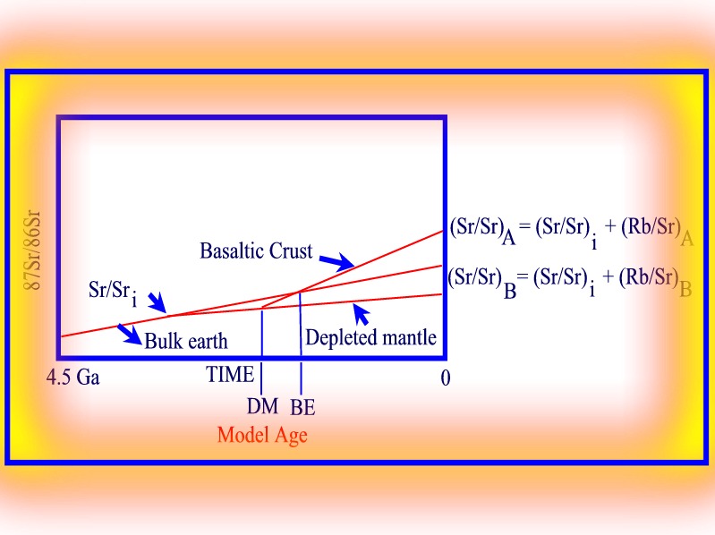
As illustrated in the following diagram, solving for delta t in the simultaneous equations is equivalent to determining the point of backward intersection of the the sample and Bulk Earth Sr/ Sr growth curves in a plot of Sr/Sr against Time. The age at the point of intersection is known as a 'model age' and is considered to represent the maximum age the basaltic material can have based on the assumption of either a Bulk Earth or Depleted Mantle source. Note that the Model Age relative to the Depleted Mantle will be older than the model age relative to the Bulk Earth.
87Sr/86Sr versus time - Model age.
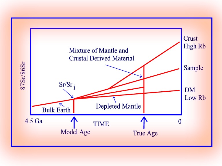
In the case of sediments or granite derived from sediments with a mixed source, the model age is the average age of the source material. In this case all that can be said is that the age of the sediment must be younger than its model age. The true age of the sample, determined by some other method e.g. U-Pb in zircon, could be considerably younger than its model age, in which case it would be necessary to contemplate an origin in terms of mixing mantle derived material with a crustal component with higher Rb/Sr and Sr/Sri values.
87Sr/86Sr versus time - model age by mixing.
Th/U-Pb
206Pb,
207Pb and 208Pb are
produced by the radioactive decay of 238U, 235U and 232Th, respectively.
The only non-radiogenic isotope of lead is 204Pb, and the isotopic composition
of lead is therefore usually expressed as 206Pb/204Pb, etc, e.g.
(206Pb/204Pb)T = (206Pb/204Pb)i + (238U/204Pb)tn
(e^l.dt - 1)
The
main advantage of using zircon to date rocks is that zircon can be assumed
to contain no initial lead,
and the age equation reduces firstly to :
(206Pb/204Pb)T = 238U/204Pb (e^l.dt -
1)
and then to
206Pb/238U = (e^l238.dt - 1)
For the nuclide pair 235U-207Pb, the equation would
be :
207Pb/235U = (e^l235.dt - 1)
AND
206Pb/238U = 207Pb/235U ((e^l238.dt
- 1)/(e^l235.dt - 1))
Zircon ages are usually calculated using what are called 'Concordia Diagrams' involving plots of 207Pb/235U against 206Pb/238U, and where the concordia line is respresented by the latter equation. Distance measured along the line from the origin is a measure of the age of the zircon, and if the zircons have not suffered chemical disturbance they should plot on the line. The age of the zircon is then said to be concordant. If the data points do not plot on the concordia line, they are said to be discordant. In this case related zircons may plot on a straight 'mixing' line, such that the upper intercept of the line with the concordia line would represent the primary age of the zircon and the lower intercept the age of some subsequent metamorphic effect.
Re-Os
In the case of the siderophile
parent-daughter pair 187Re-187Os (most of the Re - Os resides in the core),
melting of the mantle causes Re to be largely partitioned into the basaltic
melt but Os to be retained in the mantle. Following a mantle melting event
therefore, Os will grow at a much faster rate in the crust than in the
depleted mantle. 187Os/188Os of the chondritic mantle is about 0.13, whereas
187Os/188Os of the highly radiogenic crust is about 1.7. It is therefore
relatively easy using Os isotopes to differentiate melts derived from the
depleted mantle from those derived from basaltic crust.
Re-Os isotope studies
indicate that the upper part of the lithospheric mantle beneath continental
southern Africa was depleted by melting during the early Archean (low 187Os/186Os
initial) and that the diamond bearing South African kimberlites represent
small melts of enriched mantle below the radiogenic Os depleted mantle;
that the Sudbury Irruptive was formed by melting of continental material
rather than the mantle, and that the 1 billion year old Keweenawan lavas
of the Lake Superior region include a component of mantle material highly
depleted during the Archean. (Example reading: Asmerom, Y. and Walker,
R.J., 1998. Pb and Os isotopic constraints on the composition and rheology
of the lower crust. Geology, 26, 4, 359-362.)
Sm-Nd
The parent - daughter pair 147Sm - 143Nd can be treated
in the same way as Rb - Sr. However because depleted mantle is light REE
depleted (REE pattern has positive slope), and the Bulk Earth (source of
WP or Plume basalts) light REE enriched (REE pattern negative slope), and
given that Nd is lighter than Sm, melts derived from the Depleted Mantle
(high Sm/Nd) will tend to exhibit time integrated 143Nd/144Nd values greater
than melts derived from Bulk Earth compositions (low Sm/Nd).
The (143Nd/144Nd)initial
values of melts derived from the mantle can be expressed in terms of the
Nd/Nd value for the BULK EARTH in the same way that oxygen isotopes are
expressed relative to seawater, viz, eNd = (Nd/Ndsample
- Nd/NdCHUR)/Nd/NdCHUR * 10^4 °/°° where CHUR stands for Chondritic
Undepleted Reservoir The eNd values of present-day
MORB are about 8 - 12, indicating that the mantle source of MORB is depleted
relative to the Bulk Earth (Chondrite). The eNd
of a rock is calculated using the Nd/Nd values of the sample relative
to the Bulk Earth at the time of formation of the rock sample.
Variation of Nd/Nd versus time compared with eNd versus time for the mantle and crust - epsilnd.jpg
If a similar index is calculated for (Sr/Sr)initial, the data may be plotted on an eNd versus eSr diagram. On such a diagram melts derived from a depleted mantle will have positive eNd values and negative eSr values, and the melts will tend to lie along a line with negative slope passing through the value for the Bulk Earth.
A mixing line for this graph, e.g. MORB - Crust, can be calculated on the basis of the mixing equation:
[87Sr/86Sr]MIX = (X * [87Sr/86Sr]crust + (1-X) * [87Sr/86Sr]morb * Srmorbt/Srcrustt) / (X + (1 - X) * Srmorbt/Srcrustt)
Problems: Given that rock sample A has 87Rb/86Sr = .04921 and 87Sr/86Sr(Total) = .70321, and the decay constant is 1.42x10(-11)/yr, if 87Sr/86Sr(Initial) of sample A = .7018, determine t, the age of the rock.
Present day isotopic ratios for the Bulk Earth (mantle) are 87Sr/86Sr=.7045 and 87Rb/86Sr=.0827.
If rock sample A was formed as a result of melting of the Bulk Earth mantle, determine the age of the melting event.
Note: the 87Sr/86Sr of rock A and the Bulk Earth at the time of melting is not known. However, at the time of the melting event, the source mantle, the residual mantle, and the basalt will have the same 87Sr/86Sr ratio.
ans: .70321 = Sr/Srt0 + .04921(e[1.42x10(-11)xt)] - 1)
ans: .7045 = Sr/Srt0 + .0827 (e[1.42x10(-11)xt)] - 1)
ans: .70321 = t0 + .04921(e[1.42x10(-11)xt)]) - .04921
ans: .7045 = t0 + .0827 (e[1.42x10(-11)xt)]) - .0827
ans: .00129 = .03349(e[1.42x10(-11)xt]) - .03349
ans: .03478 = .03349(e[1.42x10(-11)xt])
ans: 1.038518961 = e[1.42x10(-11)xt
ans:
t = 2.66x10(9)
Model the variation in e Sr87/86 and e Nd143/Nd144 between a continental source with Sr87/Sr86 = srsrg and Nd143/Nd144 = ndndg, and basalt with Sr87/Sr86 =srsrb and Nd143/Nd144 = ndndb; where Srbasalt/Srgranite= srbsrg and Ndbasalt/Ndgranite = ndbndg, in proportions ranging from 0 to 100 percent granite.
Equations: srsrg = .706: srsrb = .702; srbsrg=.142857
srsrmix(r) = (x*srsrg + (1-x)*srsrb*srbsrg)/(x+(1-x)*srbsrg)
e srsr(r) = (srsrmix(r)/.7045-1)*10000
ndndg = .5124: ndndb = .5134; ndbndg = .16666667
ndndmix(r) = (x*ndndg + (1-x)*ndndb*ndbndg)/(x+(1-x)*ndbndg)
e ndnd(r) = (ndndmix(r)/.51262-1)*10000
Values used in the above equation are from Anderson,
p. 202, Table 10-2.
Excel solution is in: earthnt/public/300/isomix6.xls; c:\aacrse\300\rtf\isomix6.xls; c:\aacrse\330\ex\mix6.xls
To learn more about mixing click here.
FIGURES
Structural Provinces of North America.
RETURN TO:
Click here to return to beginning.
Click here to return to course outline.
Click here to return to course list.
Carbon
isotopic composition of Neoproterozoic glacial carbonates as a test of
paleoceanographic models for snowball Earth phenomena.
AU: Kennedy-Martin-J; Christie-Blick-Nicholas;
Prave-Anthony-R
SO: Geology (Boulder). 29;
12, Pages 1135-1138. 2001. .
PB: Geological Society of
America (GSA). Boulder, CO, United States. 2001.
PY: 2001
AB: Consistently positive
carbon isotopic values were obtained from in situ peloids, ooids, and stromatolitic
carbonate within Neoproterozoic glacial successions in northern Namibia,
central Australia, and the North American Cordillera. Because positive
values continue upward into the immediately overlying postglacial cap carbonates,
the negative isotopic excursions widely observed in those carbonate rocks
require an explanation that involves a short-term perturbation of the global
carbon cycle during deglaciation. The data do not support the ecological
consequences of complete coverage of the glacial ocean with sea ice,
as predicted in the 1998 snowball Earth hypothesis of P.F. Hoffman et al.
In the snowball
Earth hypothesis, the postglacial cap carbonates
and associated -5% negative carbon isotopic excursions represent the physical
record of CO2 transfer from the high-pCO (sub 2) snowball atmosphere (
approximately 0.12 bar) to the sedimentary reservoir via silicate weathering
in the snowball aftermath. Stratigraphic timing constraints on cap carbonates
imply weathering rates of approximately 1000 times preglacial levels to
be consistent with the hypothesis. The absence of Sr isotopic variation
between glacial and postglacial deposits and calculations of maximum weathering
rates do not support a post-snowball weathering event as the origin for
cap carbonates and associated isotopic excursions.
Discussion between Christie-Blick and Hoffman , March 1999 at http://www.sciencemag.org/cgi/content/full/284/5417/1087a
Christie-Blick
If highly depleted carbon isotopic values of
cap carbonates are the result of the collapse of primary productivity,
then maximum depletion of the ocean as a whole ought to date from the time
at which the ocean was frozen. However, in Namibia (1, 5), isotopic depletion
increases up section from the base of the cap carbonate (a trend that is
typical of Marinoan cap carbonates) (5, 11). Hoffman et al. ascribe this
trend to isotopic fractionation associated with the hydration of atmospherically
derived CO2 in the surface ocean, with depletion returning to bulk oceanic
values as the amount of CO2 in the atmosphere subsided from ~0.12 to 0.001
bar. This interpretation requires the ocean to have remained effectively
lifeless for an unduly long span after snowball conditions had ceased--comparable
to the duration of Marinoan deglaciation in Australia, including whatever
time was needed for the drawdown of CO2 by continental weathering (104
to 106 years?) (12) and for deposition of the cap carbonates (<105 years)
(13).
Hoffman
Christie-Blick et al. also question our interpretation
of low carbon isotopic (13C) values in the cap carbonate above the glacial
deposits, asserting that they require the ocean to be essentially lifeless
for an extended time period after snowball conditions had ceased. The 13C
value of marine carbonate reflects the relative amounts of carbonate carbon
and organic carbon burial in sediments. In our hypothesis, the low 13C
values reflect high rates of carbonate precipitation resulting from intense
chemical weathering in the extreme greenhouse conditions following the
melting of sea ice. If the rate of alkalinity delivery to seawater, and
hence carbonate accumulation, was very high, recovery of biological productivity
could be instantaneous after the deglaciation, and reach levels even greater
than modern, but still not affect significantly the 13C values of the cap
carbonates.
TI: Post-glacial carbonates of the Adrar region,
Mauritania, and the snow-ball Earth hypothesis.
AU: Shields-Graham-A
BK: In: Geological Society
of America, 1999 annual meeting.
BA: Anonymous
SO: Abstracts with Programs
- Geological Society of America. 31; 7, Pages 487. 1999. .
PB: Geological Society of
America (GSA). Boulder, CO, United States. 1999.
PY: 1999
AB: In Mauritania, 7 m-10
m periglacial polygons cap Neoproterozoic-Cambrian tillites and represent
the last traces of the cold, arid climate that led to continental glaciation
across the whole of West Africa (Deynoux, 1980). Draping these polygons
is found the thin, enigmatic dolostone that forms the subject of this presentation.
The Jbeliat cap-dolostone is mechanically laminated with scoured bedding
surfaces, and sheet, polygonal, and tepee-like dessication cracks. Barite
is present as syndiagenetically contorted veins, cavern fills, crystal
fans, and clusters of acicular crystals and is the subject of an ongoing
geochemical study (Nd-Sr-C-O-S isotopes). Volcanically derived beds with
marine calcite cements, glauconite and
phosphate occur above a significant hiatus. Below
this hiatus, dolostones yield C-isotope values between -3.7 per mil and
-2 per mil, while values are consistently positive above the hiatus. How
does the Mauritanian cap bear on the snowball question? The snowball hypothesis
(Hoffman et al., 1998) actually contains two quite different hypotheses:
1) equatorial glaciation, and 2) biopump failure (low C-isotope values).
The West African craton is likely to have been at high southern latitudes
and so has little relevance regarding the first hypothesis applied to this
particular glaciation (Marinoan?, Ediacarian?). Anomalously
low C-isotope values from Mauritania are similar to published data from
other post-glacial carbonates, but are also identical to seawater values
from the early Cambrian that are not associated with faunal extinction,
implying that other factors have been overlooked that might lower seawater
C-isotope ratios. In future studies, it will be necessary to 1) correlate
Neoproterozoic glaciations better (e.g., using Sr isotopes) so that we
can be sure that we are comparing the same event, 2) constrain the length
of the negative C-isotope excursion and the possible effect of ocean stratification
on C isotopes, and 3) apply more sensitive geochemical proxies (e. g.,
Nd isotopes).
TI: Geochemical and isotopic implications of the
snowball Earth hypothesis.
AU: Schrag-Daniel-P; Hoffman-Paul-F;
Bowring-Samuel-A
BK: In: Geological Society
of America, 1999 annual meeting.
BA: Anonymous
SO: Abstracts with Programs
- Geological Society of America. 31; 7, Pages 372. 1999. .
PB: Geological Society of
America (GSA). Boulder, CO, United States. 1999.
PY: 1999
AB: The Snowball Earth hypothesis
proposes that Neoproterozoic glacial deposits and associated "cap" carbonates
represent a series of global glaciations followed by extreme greenhouse
conditions. In the context of the hypothesis, a runaway ice-albedo feedback
causes a global glaciation, with near-complete sea-ice cover, and a greatly
reduced hydrologic cycle dominated by sublimation. Escape from this frozen
state requires several to several 10's of millions of years for carbon
dioxide, released by magmatic outgassing, to build up in the ocean/atmosphere
system, providing adequate radiative forcing to overcome the high planetary
albedo. Meltback would be extremely rapid (i.e., hundreds of years), transforming
the
earth from frozen to ultra-greenhouse
conditions. The hypothesis predicts that the cap carbonates were rapidly
deposited, with alkalinity supplied by intense carbonate and silicate weathering.
An important question is whether carbonate dissolution during the glaciation
was sufficient to maintain carbonate saturation. If so, then the rapid
warming of the surface ocean would also drive massive carbonate deposition
at a global scale, followed by continued deposition at lower latitudes
due to weathering. The carbon isotopic compositions of the cap carbonates
are consistent with this hypothesis. Values immediately on top of the glacial
deposit are between 3 and 0 per mil, consistent with dissolved inorganic
carbon in isotopic equilibrium with a CO (sub 2) -rich atmosphere. Values
rapidly decrease to 5 per mil, consistent with Rayleigh distillation of
the atmosphere as carbonate is deposited, and mass balance considerations.
Elevated (super 87) Sr/ (super 86) Sr values above the basal carbonate
unit are biased by
in-situ Rb decay, but are
consistent with very intense weathering of silicate rock flour after an
initial sequence of carbonate deposition due to degassing of seawater during
ocean warming and/or intense carbonate weathering prior to eustatic sea-level
rise from melting continental glaciers. The reasons why the Earth was susceptible
to such glaciations in the Neoproterozoic (and possibly the Paleoproterozoic)
remains a mystery, but the assembly of large continents at low-latitudes
may have been a contributing factor to achieving low atmospheric CO (sub
2) by reducing the negative feedback of ice-cover on silicate weathering
of continents.
TI: Neoproterozoic low-latitude glaciation and
the snowball Earth hypothesis.
AU: Hoffman-Paul-F
BK: In: Geological Society
of America, 1999 annual meeting.
BA: Anonymous
SO: Abstracts with Programs
- Geological Society of America. 31; 7, Pages 371-372. 1999. .
PB: Geological Society of
America (GSA). Boulder, CO, United States. 1999.
PY: 1999
AB: The occurrence of late
Neoproterozoic glacial deposits on every continent led Harland (1964) to
postulate a global ice age. Simple energy-balance climate models (e.g.,
Budyko, 1969) suggested that runaway ice-albedo feedback might occur if
solar luminosity or greenhouse gas concentrations were substantially diminished.
These findings were not taken seriously at first because there seemed to
be no means of recovery from the high albedo of an ice-covered Earth and
it was thought that all life would be extinguished. Caldeira and Kasting
(1992) later estimated that recovery would be possible if atmospheric CO
(sub 2) levels rose to approximately 0.12 bar (350x present), which could
result from normal volcanic
outgassing over millions of years in the absence
of sinks for carbon (i.e., no photosynthesis or silicate weathering). Reliable
paleomagnetic evidence that ice lines reached sea level near the equator
during the Marinoan ice age in Australia led Kirschvink (1992) to invoke
an albedo-driven "snowball" Earth. He noted that global sea ice would limit
air-sea gas exchange, leading to anoxic oceans rich in dissolved iron,
explaining the co-occurrence of Neoproterozoic iron-formations and glacial
deposits. My coworkers and I (1998) pointed out that petrographically distinctive
"cap" carbonates and large negative d13C anomalies, both widely associated
with Neoproterozoic glacial deposits, could be explained by a snowball
Earth
and its ultra-greenhouse aftermath. Thus, the
snowball Earth hypothesis is well grounded in theory (climate models),
well supported by a variety of geological evidence (e.g., sea-level ice
line near the equator, iron-formations with ice-rafted dropstones, "cap"
carbonates with large negative d13Canomalies, large sea-level changes),
and makes testable predictions concerning its longevity and its ultra-greenhouse
aftermath. Moreover, as originally noted by Martin Rudwick (1964), the
snowball hypothesis provides a new perspective on the longstanding problem
of the origin of metazoa. An evolutionary burst might be expected
to result from the imposed series of population bottleneck-and-flush cycles,
with severe genetic isolation during glaciations and unique transient selective
environments at times of repopulation. The severity of these events may
be judged from the long basal stem of eukarya in universal phylogenetic
trees based on molecular sequencing.
AN: 2001-023924
TI: The Paleoproterozoic snowball Earth; cyanobacterial
blooms and the deposition of the Kalahari manganese field.
AU: Kirschvink-Joseph-L; Gaidos-Eric-J;
Beukes-Nic-J; Gutzmer-Jens
BK: In: Geological Society
of America, 1999 annual meeting.
BA: Anonymous
SO: Abstracts with Programs
- Geological Society of America. 31; 7, Pages 372. 1999. .
PB: Geological Society of
America (GSA). Boulder, CO, United States. 1999.
PY: 1999
AB: Geological, geophysical,
and geochemical data suggest that Earth experienced several intervals of
intense, global glaciation ("snowball Earth" conditions) during Precambrian
time, including at least one event in the Paleoproterozoic and perhaps
four events during the Neoproterozoic. The abrupt, greenhouse-induced termination
of these events would lead to the rapid deposition of both banded iron
formations (BIFs) and cap carbonates. However, melting of the oceanic ice
should also induce an immediate and massive bloom in the cyanobacteria,
as deep-sea hydrothermal vent fluids are remarkably similar in composition
to the nutrient media needed for cyanobacterial growth. This "green Earth"
condition should produce an oxygen spike in the euphotic zone leading to
the oxidative precipitation of ferric iron followed by manganese. We show
that a particularly severe Paleoproterozoic snowball Earth at approximately
2.4 Ga would produce the geological pattern observed in the economically
important Paleoproterozoic Kalahari Manganese Field (KMF) in Southern Africa.
A newly-discovered drop-stone layer at the base of the Hotazel Formation
(which contains the KMF) argues that the low-latitude glacial interval
signaled by the Makganyene diamictite - Ongeluk volcanic sequence broke
up just prior to KMF deposition. Due to the lower solar luminosity at this
time, nearly 0.6 bar of CO (sub 2) would be needed in the atmosphere to
break the snowball condition, which would require between 35 and 70 Myr
to build up (at the present and twice the continental outgassing rates,
respectively). If this scenario is correct, it represents a singular event
in Earth history of a magnitude dwarfing later catastrophes such as the
Cretaceous-Tertiary impact.