Click here to go to 'Figures/Overheads' section.
Click here to return to course outline.
Click here to return to W.R. Church's home page.
Click here to return to Earth Science course list.
[Note: a Byte binary file is a
binary image file in which all cells have values within the range of 0
to 255 (positive only) and can thus be stored as single-byte integers rather
than the two-byte integers normally required. Byte files take half the
disk space required for normal integer files and may be created with CONVERT.
In cases where the conversion involves a change from real numbers to either
integer or byte, you will be offered the choice of conversion by truncation
(fractional portions are chopped off) or by rounding.
If the conversion results
in a packed binary file (run-length
encoded) and the resulting data values fall within the range 0 -
255, the data type will be forced to byte regardless of the initial type
chosen, and a message will appear.
Conversion of integer files to a packed binary format does not always
lead to data compaction. The packed binary format is by run-length encoding.
The image is therefore stored as a series of number pairs with the first
number indicating the run or number of repeats and the second number indicating
the attribute code or data value. If the image contains many areas of the
same value such as with most map data, then the runs will be large and
the packed binary format will lead to substantial compaction. If most cells
tend to have different values from their neighbors such as with satellite
imagery or digital elevation models, then the runs will be small and the
compaction will be minimal or absent -- indeed, the resulting file may
even be larger than the original! If you are in doubt about the efficacy
of using CONVERT to pack a file, try it! The procedure is fast enough to
compare the compacted file size with the original, and if it doesn't help,
use CONVERT to decompress it back to its original form.]
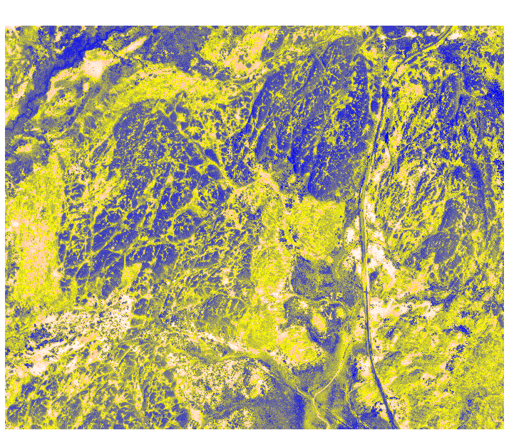
A palette might be formulated such that water would be represented by a colour range from black to dark blue, snow by a range from pink to white, vegetation by a range of colours in green and/or orange, and rocks in a range of colours in cyan, magenta, yellow and red. Since the grey scale ranges for different objects will overlap, it will require some experimentation to formulate an optimized palette, and the palette will need to be customized for each photograph to be coloured. Although the certainty of identifying objects on the basis of their grey scale value is subject to the limitations imposed by overlapping values for different objects, the addition of colour can help to differentiate non-random variation within the range of grey scale values represented by the photograph. The procedure used in this exercise is similar to that used in the classification of objects in remote sensed images (LANDSAT, SPOT, RADARSAT). Such images are low resolution (10 - 30 metres) compared to air photos, but have a much greater range of spectral information. The exercise will use a pair of stereo photographs of the 3rd year field camp area north of Coniston, Sudbury. Rock units displayed on the photographs include Mississagi Quartzite, large bodies of intrusive Nipissing gabbro, and Sudbury breccia, as well as snow, vegetation, bog and water. The images represent about one quarter the area of a standard 9 x 9 inch airphoto. The photos were digitized at 600 dpi, and each image file has a size of about 6 Megabytes. Reducing the resolution to a half (300 dpi) diminishes the file size to one quarter, i.e. digitizing a whole airphoto at 300 dpi requires about 6 Megabytes of disk space.
Operation:
1) Mapping a Network drive
Map a drive letter to the path 'Earthnt/Public/' ONLY if this operation has not already been carried out.
Map a drive letter to the path 'Earthnt/Public/' by carrying out the following instructions:
Fetch NT Explorer - click Start -> Programs -> Windows NT Explorer
Click Tools in the Toobar
Click 'Map Network Drive'
Click 'Earthnt', and then 'Public'.
Click OK
This will set a drive letter for the path 'Earthnt\public\
2) Colour classify the different grey scale components of the image
Load Idrisi and set the environment to the 'mapped drive'\300b\image, i.e. Earthnt\public\300B\image.
Display the airphoto image 4621-12b with a 256 grey scale palette.
Using the Query tool, the icon with the '?' in the IDRISI toolbar, and click on variously 'greyed' parts of the photograph to determine the range of grey values representing the various components of the image, e.g. various shades of white snow might be represented by values between 200?? and 255; water, tree clumps, and soot covered gabbros by values between 0 and 80??; light rocks and vegetation between 80?? and 200??, etc.
Fetch the Palette Workshop and 'Save As' the palette in the 'Working Directory' (click the 'Save in Working directory' button) with the name pal'your intials1'.
Use the Palette blend function to attribute to each component of the image its own range of colours - at this point request help from the instructor on how to create palette colours and how to blend end-member colours. Save the modified palette.
Create another palette pal'your intials2' that will 'block colour' rather than blend the various ranges of grey shade.
3) How to generate a digitized vector image.
The following instructions concerning the digitize operation has been taken from the IDRISI Help file. Read these notes first and then carry out the instructions
************************************************************************************************************************
DIGITIZE Operation
In order to digitize on screen, the map window you wish to digitize must have focus. Clicking on the DIGITIZE button (shaped like a cross in a circle) on the toolbar will bring up the dialog box. You must first enter a name for the vector file to be created. Then you must specify the type of feature to be digitized (point, line or polygon). You are also required to enter the feature ID (identifier) to be used for the first feature to be digitized. You may enter any positive integer value here. In addition, if the vector layer type is a point layer, you will need to enter the step value. (See DIGITIZE Note 1.) Finally, give the vector file a title. Press OK and you may begin digitizing.
To digitize, use the left mouse button to identify points that define the position, course or boundary of a feature. You will notice it being formed as you digitize. To finish the feature (or the current sequence of points in the case of point features), click the right mouse button.
Note very importantly that many of the interactive screen options will become inactive (and will thus appear grey on the toolbar) while you are digitizing. To restore them, you must terminate the feature you are working upon by clicking the right mouse button while it is on the map window concerned.
To delete an entire feature, you can click on the DELETE button -- -- to the immediate right of the DIGITIZE button). If you are currently digitizing a feature, this will cause it to be erased from the screen and be deleted from the vector layer data file. If you are not currently digitizing a feature, but have not yet closed the vector layer data file (see below), clicking this button will have the effect of deleting the most recently digitized feature from that file.
Once you have finished a feature by clicking the right mouse button, you can continue to add further features to the same vector layer data file. Make sure that the map window concerned has focus and then click on the DIGITIZE button on the toolbar. This dialog box requires that you specify the feature ID of the new feature, and step value if it is a point layer. You can then start digitizing again once you press OK.
As you digitize features, they will each in turn be added to the vector layer data file. In order to close this file, and stop the process of adding features to it, simply click on the SAVE button. If you do this, the next time you click on the DIGITIZE button, you will need to enter the name of a new vector layer in which to save the data.
**************************************************************************************************************************
Click the DIGITIZE
button and in the 'On-Screen Digitizing' window enter a name for the vector
file to be created, e.g. 'yourinitials'sstne. Click the POLYGON
button but leave the Feature ID as '1'. Click
OK.
Outline an area of sandstone
by sequentially clicking the left mouse button,
terminating the sequence by clicking the right
mouse button. Click the DIGITIZE button once
again and click the OK button in the Digitize
window that appears, leaving the value of the Feature
ID as '1'.
Define another area of sandstone with the left mouse button. Cick the right mouse button to close the polygon. You can continue to add as many polygons to the sstne1 file as you want. When you have finished creating polygons, click the SAVE button (the bent arrow icon second to the right of the digitize icon). The 'yourinitials'sstne file will be closed.
Overlay the new vector layer on the airphoto by clicking the Add Layer button in COMPOSER and selecting the sstne1 layer as the display layer using the QUAL16 palette. You can also display the vector image you have created with Display -> 'Display Launcher', etc.)
Repeat the operation for the gabbro but in the 'On-Screen Digitizing' window, name the file 'yourinitials'gab and give the gabbro polygons an identifier value of '2'.
4) ( How to generate an enlarged 3D image from a pair of digitized airphotos. Optional depending whether or not you are able to unfocus your eyes.)
Display the stereoscopic images 4621-12b and 4621-13a using the GARSON2 palette. Zoom the images to the area indicated by the lab instructor. Match the images to produce a stereo view of the area, and identify the folds in the Mississagi quartzite unit.
RETURN TO:
Click here to return to beginning.
Click here to return to course outline.