CTM: lsim

lsim

The lsim command is quite similar to the step command (actually, the step command is just a special case of lsim). Given a system described either by state-space equations or a transfer function, the lsim command can run a simulation of the system using arbitrary inputs and initial conditions.

The command lsim(A,B,C,D,U,T,X0) plots the time response of the linear system:

 			.
 			x = Ax + Bu
 			y = Cx + Du

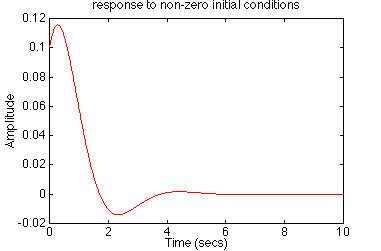
That is, the differential equation is integrated from time T(0) to T(length(T)), starting at the initial condition X0 and using the input U. The input vector must have the same number of entries as the time vector. If the initial conditions are all zero, X0 can be omitted.

Suppose we have a system described by the state space-equations above, with A,B,C,D matrices:


A = [-20   -40   -60
     1    0    0
     0    1    0];

B = [1
     0
     0];

C = [0   0   1];
D=0;

As you can see from the dimensions of the matrices, this system has three states, one input, and one output. Let's say we want to plot the response of the system with a non-zero initial condition and no input. This can be done in the following manner.

 
T = 0:0.01:10;                % simulation time = 10 seconds
U = zeros(size(T));           % no input
X0 = [0.1 0.1 0.1];           % initial conditions of the three states 
lsim(A, B, C, D, U, T, X0)    % simulate and plot the response (the output)

When the lsim command is invoked with left-hand arguments,


[Y, X] = lsim(A,B,C,D,U,T);

Matlab returns the output and state time history in the matrices Y and X respectively. No plot is drawn on the screen. The matrix Y has as many columns as there are outputs and length(T) rows. X has as many columns as there are states and length(T) rows. The plot command can then be used to plot the response.

Now let's plot the step response for the system given above; the input U is 1 for all positive time, and the initial condition is zero.


T = 0:0.01:10;                 % simulation time = 10 seconds
U = ones(size(T));             % u = 1, a step input
[Y, X] = lsim(A,B,C,D,U,T);    % simulate
plot(T, Y)                     % plot the output vs. time

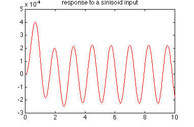
The plot above shows the step response of the system. We can also plot the response of the system to any other input that we choose. For example, if we had a sinusoidal input, say u(t) = 0.1 sin(5t+1):


T = 0:0.01:10;                  % simulation time = 10 seconds
U = 0.1*sin(5*T+1);             % input as a function of time
[Y, X] = lsim(A,B,C,D,U,T);     % simulate
plot(T, Y)                      % plot the output vs. time

Remember that the steady-state response of a linear system to a sinusoidal input will always be a sinusoid of the same frequency but with a different magnitude and phase.

This same sinusoidal response could also be found by transforming the state-space equations into the transfer function form:


T = 0:0.01:10; 
U = 0.1*sin(5*T+1);
[num,den]=ss2tf(A,B,C,D);
lsim(num,den,U,T)

You should get the same picture as above.

Because any transfer function can be represented using many different sets of state-space matrices, you can only simulate a system in transfer function form with zero initial conditions; see the conversion page for more details.

User feedback