PART E - PREREQUISITE – Earthquakes

Introduction

In PART D, we learned that segments of Earth’s lithosphere slowly move with time, driven by the heat engine of Earth’s interior. The term encompassing all interactions of those segments is plate tectonics. One serious consequence of plate interaction is earthquakes – and it would be difficult to find a natural phenomenon that strikes more fear into the heart of humans. To illustrate that point, here’s a true story!

Between 16^th December, 1811 and 7^th February, 1812 three separate series of earthquakes, totaling nearly 2000 quakes of varying intensity, occurred in the crust beneath the little town of New Madrid, Missouri (Fig. E1; the ‘intensity’ shown uses the Modified Mercalli Scale, and we’ll define it later. For now, accept that the main event at New Madrid was the top number on that scale.). The greatest of the shocks was one of the greatest ever experienced anywhere. The quake was so strong it rang the church bells in Boston, 1600 km away. It was even felt here in London. [We'll return to a discussion of the cause of the earthquake in the lecture portion of 240A]. Ever since 1812 it has been widely acknowledged that if an earthquake of that magnitude struck the same location today, it would be a tragedy of staggering proportions. In October of 1989, a climatologist by the name of Iben Browning predicted that on December 2^nd or 3^rd of 1990 a devastating earthquake would again occur in the New Madrid area. He based his prediction upon the patterns of Earth's tides - a prediction method which was beginning to be considered as an instigator of volcanic eruptions (we'll talk about that later), but had no record of reliability for earthquakes. However, the media - always keen to find a controversial item - jumped on the story and descended on the area en mass. They panicked the inhabitants! Some just packed and ran; others bought all the foodstuffs, bottled water, portable generators and tents they could find and set up in the open fields (most fatalities from earthquakes arise from collapse of buildings, so they did the right thing). Someone even imported hundreds of body bags to be ready for the expected carnage. Needless to say, there was no earthquake; the story just serves to illustrate the fear we have of them, and how poorly we can predict them.

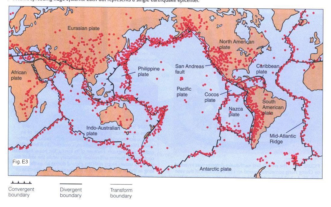
In this section we will review the types of crustal block interaction to produce earthquakes, the means we use to detect them, and how we measure their severity. To bring home the close association of earthquakes with plate interaction, look at Figure E2, and note that the vast majority of earthquakes occur right along plate boundaries. We covered the types of plate interaction that are produced by stress in PART D (Plate Tectonics). In fact, plate boundaries are seldom defined by a single break, but by a series of parallel faults. During our study of earthquakes, however, we are almost always concerned with interpreting a specific instance of activity along a specific fault. So, what follows is a much more detailed consideration of stress.

Stress and Strain

An object is under stress when force is being applied to it. The stress may be compressive, tending to squeeze the object, it may be tensile, tending to pull the object apart, or it may be a shearing stress that tends to cause different parts of the object to move in different directions across a plane (or to slide past one another, as when a deck of cards is spread out on a table by a sidewise sweep of the hand).

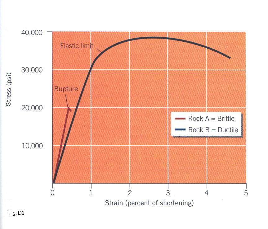
Strain is deformation resulting from stress. It may be either temporary or permanent, depending upon the amount and type of stress and the material's ability to resist it. If the deformation is elastic, the amount of deformation is proportional to the stress applied (Fig. E3), and the material returns to its original size and shape when stress is removed. A gently stretched rubber band shows elastic behavior. Rocks, too, may behave elastically, although much greater stress is needed to produce detectable strain.

Once the elastic limit of a material is reached, the material may be so brittle that it fails (breaks), or it may be sufficiently ductile that it may go through a phase of plastic deformation with increasing stress. During this plastic deformation stage, relatively small added stresses yield large corresponding strains, and the changes of shape are permanent: the material does not return to its original dimensions after removal of the stress. A glassblower, an artist shaping clay, and a blacksmith shaping a bar of hot iron into a horseshoe are all making use of plastic behavior of materials.

If stress is increased further, all solids eventually break, or rupture, as a rubber band will do when stretched too far. In brittle materials, rupture may occur before there is any plastic deformation. Brittle behavior is characteristic of most rocks at near-surface conditions and is illustrated in Figure E3 by the behavior of Rock A. At greater depths, where temperatures are higher and rocks are confined, the same rocks may behave plastically (line showing behavior of Rock B). The effect of temperature can be seen in the behavior of cold and hot glass. A rod of cold glass is brittle and snaps under stress before appreciable plastic deformation occurs, while a sufficiently warmed glass rod may be bent and twisted without breaking.

As already indicated, the physical behavior of a rock is affected by external factors, such as temperature and confining pressure, as well as by the intrinsic characteristics of the rock itself. Also, rocks respond differently to different kinds of stress. Most are far stronger under compression than under tension: a given rock may rupture under a tensile stress only 1/10^th as large as the corresponding compressive stress required to break it at the same temperature and pressure. Consequently, the term strength has no single, simple meaning when applied to rocks unless all of these variables are specified.

Faults

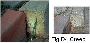
Most earthquakes are associated with sudden movements of rock along breaks or fractures called faults. By definition, a fault is a fracture in the lithosphere along which measurable movement has occurred. Realize, of course, that every time we map a fault in the field, we are mapping the evidence of an earthquake. When movement along existing faults occurs gradually and smoothly, it is termed creep. Creep causes broken curbstones (Fig. E4), offset fences, etc. In buildings, dams or other structures built directly across a fault, creep can stress and deform walls to the point of failure over a period of time. But damage is highly localized, and lives are rarely lost as a consequence of slow creep. Obviously, if we’re considering earthquakes, we’re not considering creep. Let’s consider the different fault geometries and the sort of stress-strain associated with them.

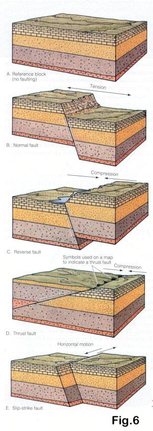
To make a normal fault (Fig. E5b

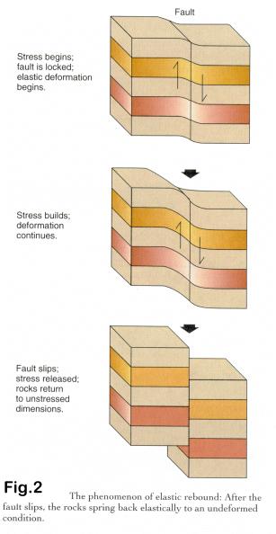
), there must be tension so that one block can move down the fault plane relative to the other. The result is extension. This is a common movement close to a spreading center. Reverse faults (Fig. E5c) are produced by compression, and a thrust fault (Fig.5d) is just a special case (where the angle is very shallow) of a reverse fault. Obviously, this must be a common feature where two plates come together. Strike-slip faults (sometimes called ‘transverse faults’; these are the faults that define a transform plate boundary) (Fig. E5e) are the result of shear movement, and the San Andreas Fault in California (Fig. E6) is probably the best know one. However, there are many other spectacular ones, such as the Great Glen Fault of Scotland (Fig. E7). There is a great marker horizon along the Great Glen Fault; a small granite intrusion that formed along the fault line some 350 million years ago has subsequently been split by the fault with the two bits now being a little over 100 km apart. There are a few very small earthquakes along the Great Glen Fault still, but most are so small that we presume most movement has stopped. By the way, note that Loch Ness is a linear lake right along the fault line. There is, as you know, a legend about some ancient creature from the dinosaur days that lives in the lake. Whatever lives in the lake, it's not from that long ago; the whole region was covered by ice 10,000 years ago, and the whole of the depression was filled with ice, not water.

Friction between rocks on either side of a fault is such as to prevent the rocks from slipping easily, or when the rock under stress is not already fractured, some elastic deformation occurs before failure. When the stress at last exceeds the rupture strength of the rock (or friction between rocks along an existing fault), sudden movement occurs: an earthquake! The stressed rocks, released by the rupture snap back elastically to their previous dimensions, a phenomenon known as elastic rebound - but they are offset (Fig. E8).

Try this simple-minded demonstration. Take a thin wood dowel and gently bend it, then hold it in the bent position; the muscle energy used to bend the wood didn't disappear simply because you stopped the motion - it is stored as elastic energy in the wood. If the ends are released, the wood rebounds to its original shape. However, when the pressure is so great that the elastic limit is exceeded, the wood breaks (watch your eyes!). The elastic energy is now converted, at least in part, to heat at the breakage point, and in part to sound waves, and in part to vibrations in the wood.

On a rather different scale, earthquake vibrations are the same kind as you felt in the wood when it broke. Just how elastic energy is stored and built up in Earth is a subject for intensive research.

The first evidence supporting the elastic rebound theory came from simple observational studies across the San Andreas Fault. Figure E9 illustrates what was seen. About 1874, a picket fence was built along the boundary of a property that straddled the fault. As time passed, the fence line was increasingly distorted into a 'z' shape as stress increased along this segment of the fault; friction along the fault plane prevented motion. On April 18, 1906, the two sides of the locked fault slipped abruptly [during the great 1906 San Francisco Earthquake!]. The elastically stored energy was released as the fault blocks moved and the bent crust rebounded. The fence on either side returned to its previously straight-line configuration - but the two segments were offset by the motion along the fault.

It’s an Earthquake!

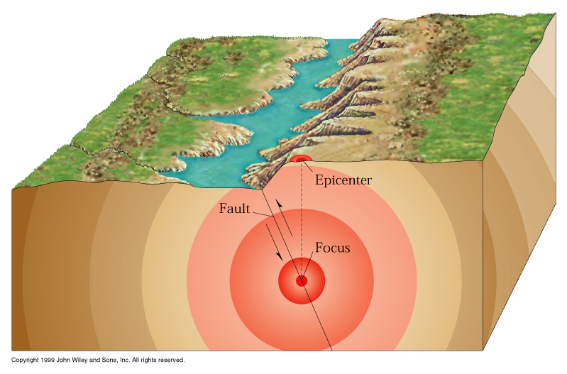
The point within Earth where the rupture starts is known as the focus or hypocenter (Fig. E10). The rupture may begin at one specific spot, but the shock of that release is usually enough to cause release all around it on the fault plane, and, for some considerable distance (until the stress is dissipated), the whole fault plane releases. The waves of energy that move outward from the point of initial disturbance are called seismic waves. Directly above the focus, on the surface of Earth, is a point called the epicenter. Earthquakes are classified as shallow-focus (0-70 km), intermediate-focus (70-300 km) or deep-focus (300-800 km), and we know that earthquakes do not occur any deeper than about 800 km (we’ll get to that later).

Seismology and Seismic Waves

In PART D: Prerequisite, we covered some of the basics of seismology; we learned that seismology is the study of shock waves - particularly earthquake shock waves - so we had better consider a bit of detail about seismic waves before we try and determine where an earthquake originates and how we express earthquake magnitude.

The elastically stored energy that is released by an earthquake is transmitted to other parts of Earth. As with any vibrating body, waves spread outward from the earthquake’s point of origin (its focus). These waves, called seismic waves, spread in all directions from the focus, just as sound waves spread in all directions from the sound source. Seismic waves are elastic disturbances, so the rocks through which they pass return to their original shapes after the passage of the waves. The waves, therefore, must be measured and recorded while the rock is still vibrating. For this reason, continuous recording seismograph stations have been installed around the world.

We already know (from PART D: Prerequisite) that seismic waves are of two main types: body waves that travel outward from the point of origin and have the capacity to travel through Earth, and surface waves that are guided by and restricted to Earth's surface. Body waves are analogous to light and sound waves; surface waves are analogous to ocean waves because they are restricted to a free surface. We need, now, to consider a bit more detail about the character of seismic waves than we did in PART D.

Body Waves

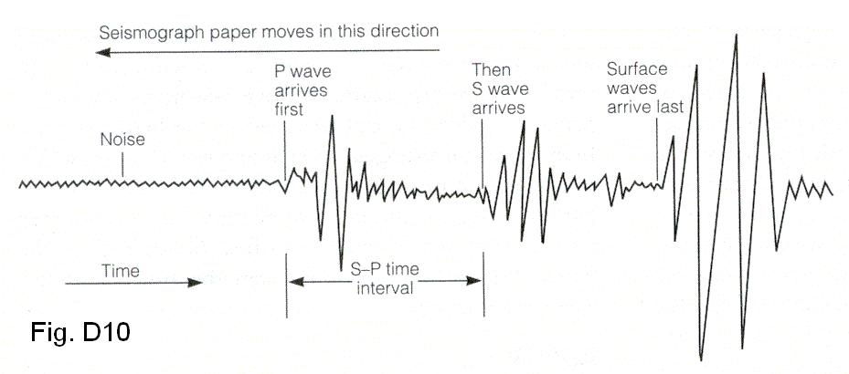
The faster body wave (average value of 6 km/s through continental crust), called a Primary (or P) wave, acts as a compression waves can pass through solids, liquids, or gases because all three can sustain changes in density (see Fig. E11: graph showing relative arrival times of P, S and surface waves). The somewhat slower Secondary (or S) body wave (average value of 3.5 km/s through continental crust) acts with a shearing motion that deforms the shape of material. Because gases and liquids do not have the elasticity to rebound to their original shape, shear waves can be transmitted only by solids.

Surface Waves

Surface waves travel along or near the surface of the Earth like waves along the surface of a body of water. They travel more slowly than either P or S waves, and they pass around the Earth rather than through it. Thus, surface waves are the last to be detected by a seismograph. There are two kinds of surface waves, just as there were two kinds of body waves. Love waves and Rayleigh waves, and we’ll see in the regular 240A lectures sequence how they are useful in interpreting earthquake magnitudes.

Seismic Wave Intensity/Magnitude

The two common scales used to measure earthquakes are: the Modified Mercalli Intensity Scale and the Richter Magnitude Scale. Although each earthquake has a unique magnitude, its effects will vary greatly according to distance from the focus, ground conditions, construction standards, and other factors. The Modified Mercalli Intensity Scale is a purely subjective indicator, while the Richter Magnitude Scale (named after Charles Richter) is based upon precise measurements of vibration recorded on instruments (seismographs).

The Modified Mercalli Intensity Scale

In seismology, a scale of seismic intensity is a way of measuring or rating the effects of an earthquake at different sites; the primary advantage is that earthquake intensity may be estimated long after the event simply because the effects will still be evident. The scale, from I to XII, is shown in Table E1. Obviously, if you rate a shock wave as VII or VIII, it's a pretty big earthquake, and a XII represents total destruction. The only earthquake in historical time which has ever rated an XII is the one with an epicenter at New Madrid, Missouri in 1811 - so you understand the potential for panic. As you can see from the list, rating the intensity of an earthquake's effects does not require any instrumental measurements. Thus seismologists can use newspaper accounts, diaries, and other historical records to make intensity ratings of past earthquakes, for which no instruments were available. Such research helps promote our understanding of the earthquake history of a region, and estimate future hazards.

The Richter Magnitude Scale

Today, seismographs are used to define both location and magnitude of earthquakes. When we discuss location (below), you’ll see that it is the epicenter that is defined; as we now discuss magnitude, note that we are defining magnitude for the focus not the epicenter.

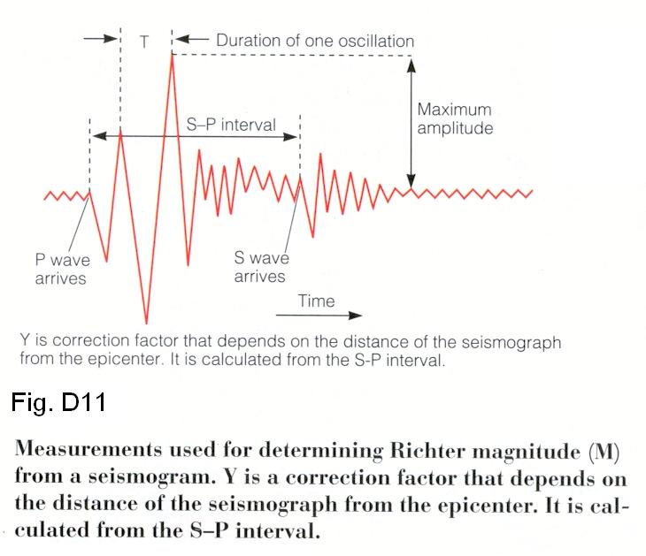
Today, there are so many seismographs sited in so many of the more populated countries that most times when we are able to use the Richter scale to indicate how big an earthquake is. The Richter scale is not linear, but logarithmic, so each unit of increasing magnitude represents a seismic wave ten times greater than the magnitude below. That means, for example, that a magnitude 7 wave has 1000 times the amplitude of a magnitude 4 wave.

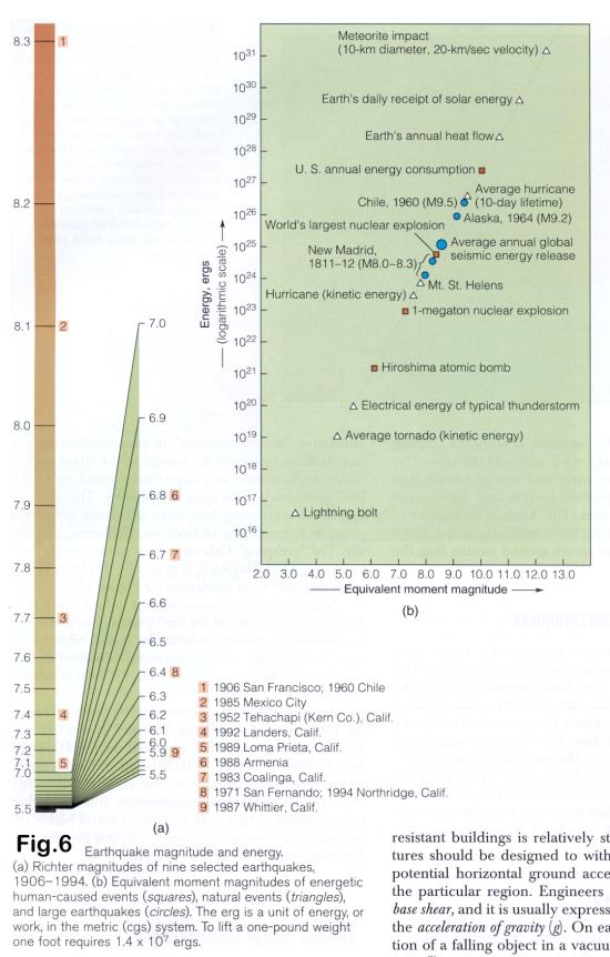
Figure E12 shows that the amplitude of any wave is its maximum height from the base level (background, or starting level). Starting with that, Charles Richter, in 1935, devised a quantitative method to record earthquake magnitudes. We will look at the details later, and the modifications to the basic technique that make it more accurate. Figure E13 shows, on a logarithmic scale, some natural and man-made seismic events; in the regular sequence of 240A lectures, we’ll consider two of the very large earthquakes illustrated: Chile 1960 at magnitude 9.5 and Alaska 1964 at magnitude 9.2.

Locating an Earthquake

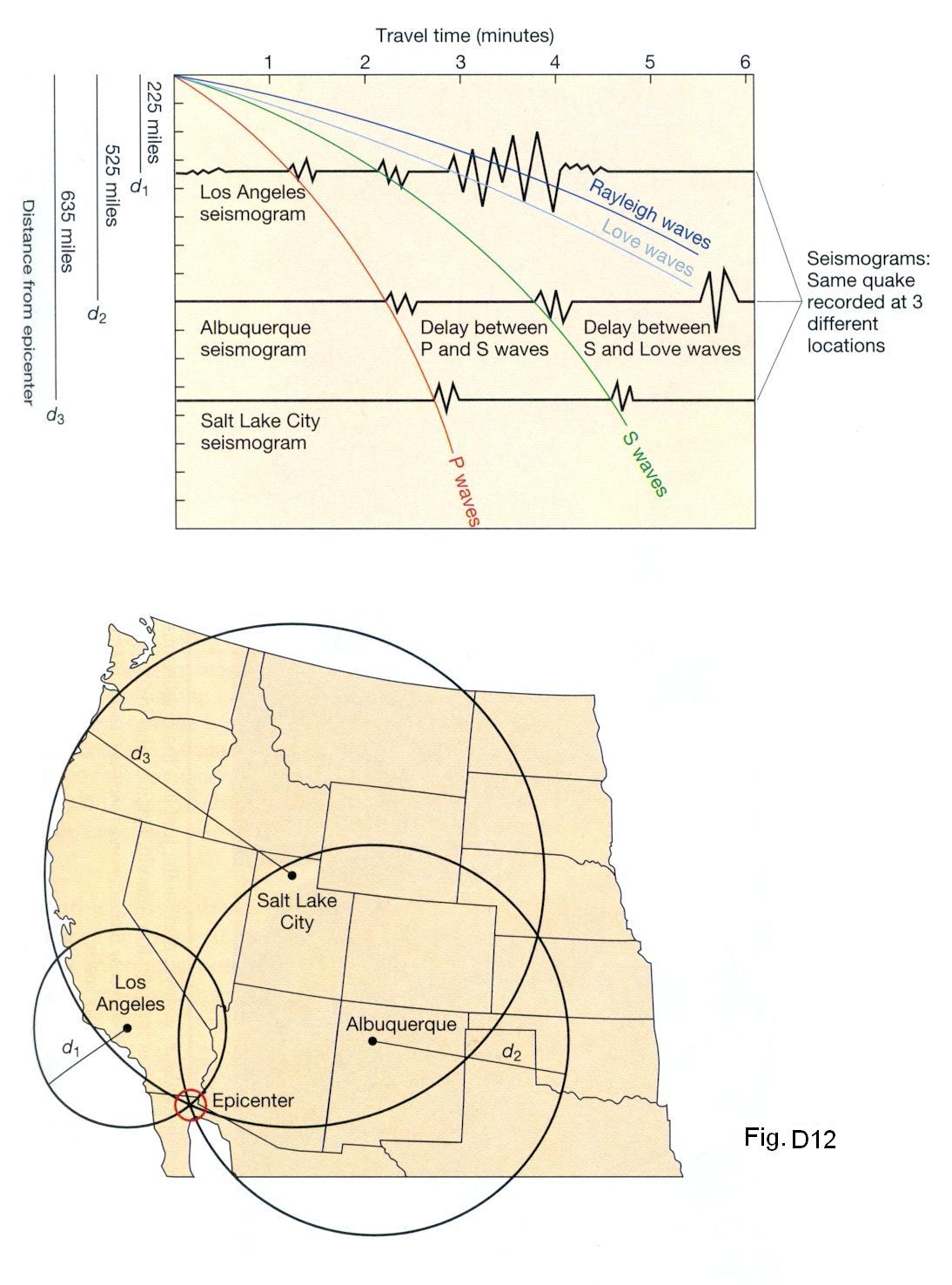
If an earthquake's waves have been recorded by three or more seismographs, its epicenter can be determined through simple calculations. The first step is to determine how far the seismograph is from the epicenter. This is done by comparing the arrival times of the P and S waves. The greater the difference between the arrival times, the greater the distance from the epicenter (as we said earlier).

Figure E14 shows the technique, called triangulation, of locating an epicenter with data from three seismographs. The seismographs are located in Los Angeles, Salt Lake City, and Albuquerque. All three seismographs show the vibration effects of the shock waves; the top schematic shows the patterns superimposed from all stations. We know the exact speed of the graph recorders, so we know the exact times of reception of the vibrations at each station. P waves arrive first at any site, and S waves second. We certainly know exactly the distances between each station, but we don't know the distance of the earthquake's epicenter from each station. To do that, we need a calibration curve - a graph which (using average crustal values for transmission speed of the different waves) correlates the difference in arrival times of P and S waves (shown in Figure 12) with distance of transmission. Figure E15 is such a calibration curve. Here, for example, if the difference in arrival times between P and S waves is about 6.3 minutes, then the seismograph is located about 4000 km from the epicenter of the earthquake. These time vs distance curves are gross approximations, based solely upon the average travel times through the crust; they could be improved provided we knew more about the materials in the area between the shock and the seismograph.

Returning to our example problem (see Figure E14), we see that the time difference for the Los Angeles station translates to 255 miles (408 km) from the epicenter, the Albuquerque station was 525 miles (840 km) away from it, and the Salt Lake seismograph was 635 miles (1016 km) away. If we now take out a decent map with exact locations of the seismographs, take a compass and draw circles around each site with radii of the numbers we just determined, then the epicenter has to be at the unique point where the circles intersect.

Please return to the regular 240A lecture sequence on earthquakes.