Click here to go to 'Figures/Overheads' section.
Click here to return to course outline.
A GIS geological mapping project involves
five stages: 1) the georegistration of existing
topographic base maps, geological maps, aerial photographs, radarsat and
satellite images, and geophysical data images, to a common grid reference
system; 2) the deconvolution (separation)
of the various classes of existing spatial
information onto a set of georegistered layers; 3) preliminary
analysis of the resulting data set; 4) ground-truthing
and further data collection in the field;
and 5) final organisation of layers and analysis
of the data.
Layering
involves the separation of data into classes in the form of georeferenced
layers. For example, the recently published data for an area
of northern Manitoba known geologically as the Flin
Flon - Snow Lake Belt (approx 250km E-W and 150km N-S) is
broken down into the following layers:
Landsat TM imagery for a 1:250k sheet - all seven
bands
Synthetic Aperture Radar (SAR) data - both airborne
and satellite for selected areas
bedrock geology maps
geological field observations, including lithological,
structural, and mineral observations
surficial geology map
quaternary data sets (clay geochem, grain size,
carbonate content striae, etc.)
digital hydrography
geophysical imagery (gravity, aeromagnetics (total
field and vertical gradient))
radiometric imagery
mineral occurrence data
geochronological data
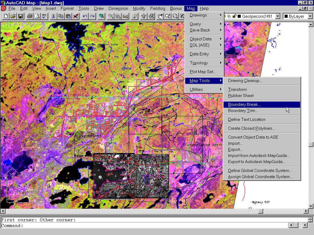
In the case of Field course 350Y, for example, the first three stages of a GIS compilation for the Coniston region of Sudbury would involve georegistration of the relevant 1:20,000 digital basemap, geological map 2491, airphoto, and aeomagnetic images, secondly, the deconvolution of the geological information (bedding and foliation orientation, faults, rock units, etc) on geological map 2491, and thirdly, analysis of the aerial photographs and remote sensed images in an attempt to, for example, predict faults, joint patterns, bedding or foliation trends, and the presence of dikes, contact metamorphic zones, or argillized zones, etc. When in the field, the predictions of the preliminary analysis can be 'ground truthed', and new data added to the spatial data base (e.g. measured dips and strikes; rock unit boundaries; sample locations, etc). Finally, with all the data assembled, the interpretive addition of rock unit boundaries and the generation of a topology and a polygon map may be attempted. The following image shows 'road' (red lines), 'railway track' (green lines), 'shoreline' (blue lines), 'town-site boundary', 'map 2491 geological boundary' (black and cyan lines), 'map 2491 bedding trend' (magenta lines) and 'bedding strike and dip symbol' layers in the Coniston/Garson region superimposed on a georegistered false-colour satellite image and two aerial photographs of part of the region. In this module we will attempt to carry out the first three stages in preparation for the 350y field course.
Which Map is Best? - Projections for World Maps, 1986, 14 p., Special Publication
No. 1, Committee on Map Projections of the American Cartographic Association
(ISBN 0-9613459-1-8). (Not in Library)
Choosing a World Map -
Attributes, Distortions, Classes, Aspects, 1988, 15 p., Special Publication
No. 2, Committee on Map Projections of the American Cartographic Association
(ISBN 0-9613459-2-6).
Matching the Map Projection
to the Need, 1991, 30 p., Special Publication No. 3, Committee on Map Projections
of the American Cartographic Association (OSBN 09613459-5-0).
Snyder, J.P. 1984, Map
Projections used by the U.S. Geological Survey, Washington: U.S. Geological
Survey Bulletion 1532, 313p. (Call # US1 IN2 82B32; TAY govt 28 day).
Peter Richardus and Ron.
K. Adler, 1972, Map projections for geodesists, cartographers and
geographers. North-Holland Pub. Co., Amsterdam. ( Call #
GA110.R52, DBW stack 28DAY)
Snyder, P.J., 1984, Map
Projections - A working manual. US Geological Survey Professional Paper.
US Dpt. of the Interior 1395,100 p. (Call # US1 IN47 84P95
TAY govt 28DAY; US1 IN47 84P95 DBW govt 14DAY)
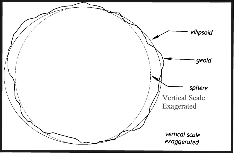
Geodesy
is concerned with the area and shape of the Earth, and in particular the
definition of a reference Earth shape known as the Geoid.
The Geoid is
an equipotential surface of gravity, ellipsoidal (oblate spheroid) in shape
because of the counter-gravity centrifugal forces generated by the spin
of the Earth about its N-S axis, and highly irregular because of the variability
in composition (density) of the Earth beneath each point on the Geoid (note:
the irregularities are not coincident with those exhibited by the Earth's
surface). The ellipsoid
model of the Earth attempts to define its shape in terms of a smooth ellipsoid,
and the use of satellite measurments have led to the development of the
WGS-84 (World Geodectic System) ellipsoid as the best ellipsoidal representation
of the Geoid. The maximum difference between the Geoid and the WGS-84 ellipsoid
is 1 in 100000 (100 metres). Ellipsoids have also been constructed
for individual continents and countries because different ellipsoids give
better fits to the Geoid at different locations, e.g. the Clarke 1866 ellipsoid
for the United States.
The
Geoid and Ellipsoid
The Ellipsoid information, an initial location
(origin), an initial azimuth (the direction of north), and the distance
between the Geoid and the Ellipsoid at the initial location defines a permanent
reference surface known as a 'Datum'. For example, the NAD-27 datum
(North American Datum , 1927 ) is based on the latitude and longitude of
Red Falls, Iowa, whereas the WGS-84 ( World Datum, 1984) is based on measurements
made from space, beyond the effects of local variations in gravity. Each
datum embodies its own concept of latitude and longitude, and at
any given locality, changing the datum may change a coordinate reading
by several hundred metres; in the Sudbury region the difference in UTM
latitude between NAD-27 and NAD-83 is 223 metres. When giving a coordinate
location it is therefore always necessary to also give the datum being
used.
Geodetic (geographic) coordinates are given in
terms of latitudinal degrees measured relative to the equator and and longitudinal
degrees measured relative to either east or west of the prime meridian
running through Greenwich, England.
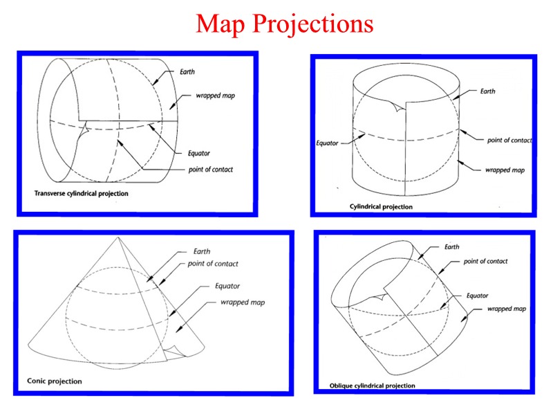
Kinds of Map Projection
Map projections involve the transformation of
a 3-dimensional form into a 2-dimensional plane; they record the curved
surface of the Earth on a flat display. They may be cylindrical, conical
or azimuthal (planar).
Cylindrical
and Conical Map Projections
As illustrated in the previous linked figure,
a cylindrical projection can be realized by
wrapping a sheet of paper around the globe, in the form of a cylinder,
projecting the geographical features onto the paper, and then unrolling
the paper as a flat sheet. Note that the great circle of contact with the
cylinder is the equator, and that the lines of latitude and longitude projected
along normals to the cylinder will draw as an orthogonal graticule (grid)
with the lines of longitude equally spaced but the lines of latitude unequally
spaced. Although the shape of a large area is distorted, small areas
are displayed relatively accurately . The maps are said to be conformal.
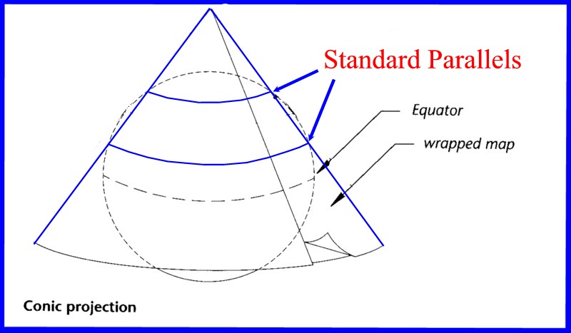
A conical
projection is generated in the same way but with the paper wrapped
as a cone such that the conical surface intersects the globe as a tangential
line of latitude, or, more usually, passes
shallowly through the globe between two small circles or latitudes
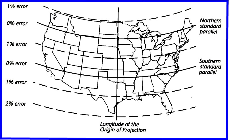
known as standard parallels (the secant case).
Standard
parallels. Lines of latitude and longitude would
in this case appear on the flattened sheet as a fan-shaped graticule, and
all features lying on the concentric circles of intersection would be undistorted.
The most common conical projection is the Lambert
Conformal Conic Projection.
Lambert
Projection
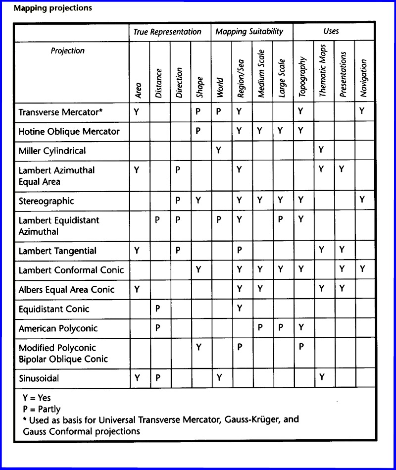
Map projections inevitably introduce distortions
of direction, area and shape into a map, and the projection to be selected
depends upon the requirements of the mapper. No map projection can offer
a uniform map scale, and projected polygonal features may retain either
their area or shape, but not both. The properties of various projections
are listed in the following link: Map
Projection Properties, Mapping
Suitability, and Uses
MAP PROJECTION SPECIFICATIONS FOR LAMBERT CONFORMAL - OGS Data set 12
The Township and Areas were digitized from hardcopy 1:50,000 scale NTS maps and assembled into an Ontario-wide fabric in Lambert Conic Conformal map projection. The following parameters define the planimetric reference grid:
Clarke 1866 ellipsoid a=6, 378,206.4 (equatorial radius) e=0.006768658 (eccentricity squared)
Standard parallels 49 degrees N latitude 77 degrees N latitude
Origin 92 degrees W longitude 0 degrees N latitude; Central Meridian 92 degrees W longitude
False Easting 1,000,000 metres
The Central Meridian at 92 degrees runs N-S just west of Atikoken, Rainy River; the western limit of the area has an easting of 750 km and the eastern limit an easting of 2500 km; the false easting origin lies approximately at the longitude of Duluth.
MAP PROJECTION SPECIFICATIONS FOR LAMBERT CONFORMAL - GSC, Geological Map of Canada
Lambert Conformal Conical Projection parameters
Type
Lambert Conformal Conic projection
Datum
North American Datum 1927 (NAD27)
Units
metres
Spheroid
Clarke, 1866
Lambert
standard parallels
49 00 00 N
77 00 00 N
Projection origin
95 00 00 W (central meridian)
49 00 00 N
False origin
(easting, northing)=(0, 0)
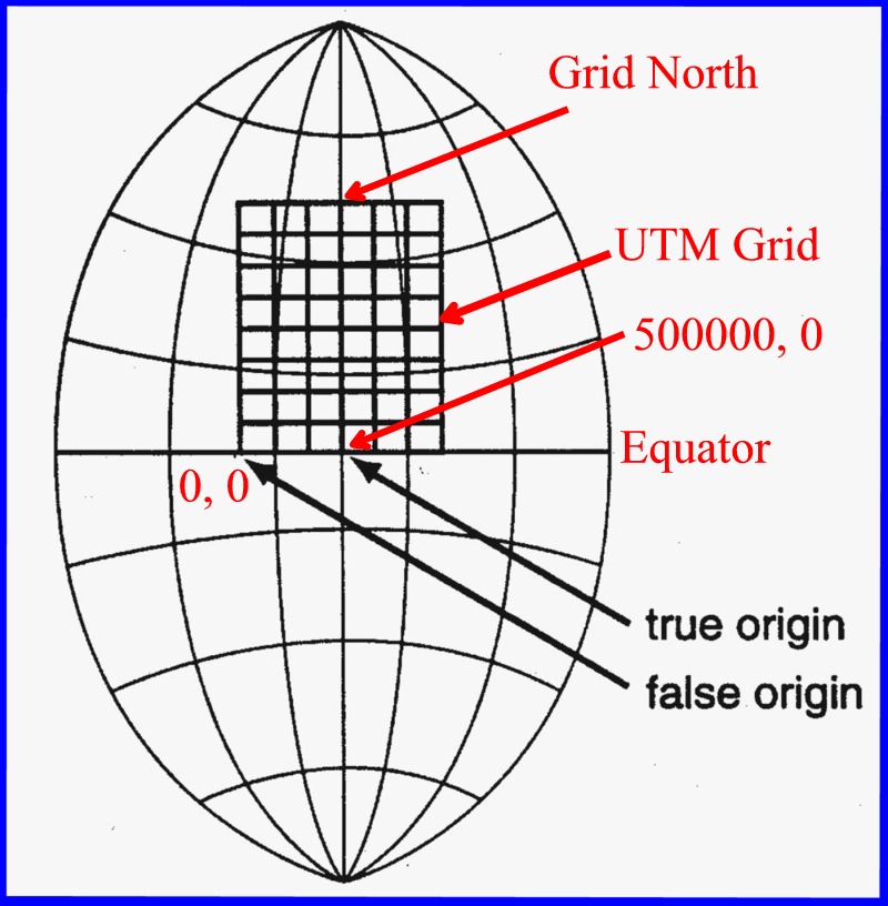
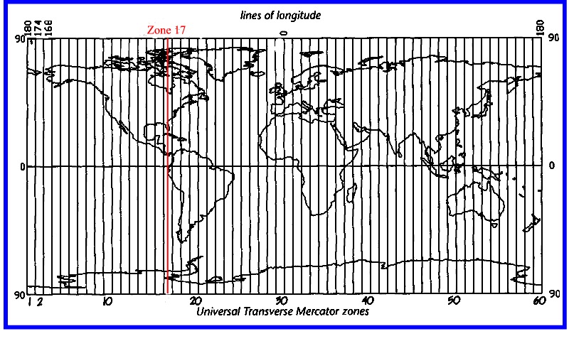
The Universal Transverse Mercator System (UTM) employs a transverse cylindrical method of projection such that distorsion is minimized along a given line of longitude, and a plane orthogonal (rectangular) coordinate system. The Earth is divided into 60 UTM zones each of 6 degrees of longitude, the zones being numbered from west to east, starting a 180W. Sudbury is located close to the centre of zone 17. The line of longitude at the centre of each zone represents Grid North, and coincides with True North. The N-S lines of the UTM coordinate grid (Eastings) are drawn parallel to Grid North, whereas the E-W lines of the grid (Northings) are drawn parallel to the Equator. The intersection of Grid North with the Equator (the true origin of the zone) is arbitrarily given a coordinate location of 500000 metres East and 0 meters North, such that a false origin for the grid, that is the point where the numbering sytem is 0 in both axes, is located 500 km west of the true origin. Note that the closer one gets to the zone boundary the larger the angular difference between True North and the UTM N-S grid line. Consequently when plotting dips and strikes of beds measured relative to Magnetic North, it is necessary to correct for this difference. At Sudbury the difference is only about 10 seconds, and therefore the correction can be disregarded.
LINKS
COORDINATE CONVERSION SOFTWARE
http://mac.usgs.gov/mac/isb/pubs/pubslists/fctsht.html
http://www.ngs.noaa.gov/PC_PROD/pc_prod.shtml#UTMS
http://everest.hunter.cuny.edu/mp/software.html
http://users.skynet.be/tandt/
http://cousin.stud.uni-karlsruhe.de/kkisbin/trafo.tcl
[In the following notes, '->' mean 'select the following option in the previously designated menu', e.g. Draw -> Point means select the Draw menu in the toolbar and then the Point menu in the presented drop-down list.]
Setting
up a Cad-based mapping project involves five main steps:
1) creating a virtual coordinate grid for the area to be studied.
2) scanning and attaching a basemap, and registering the basemap to the
virtual grid;
or attaching an existing digital map tile.
3) making the basemap transparent if not a digital tile.
4) scanning, attaching, and registering aerial photographic coverage to
the basemaps.
5) scanning, attaching, resampling any existing geological maps.
Creating Layers and a reference UTM grid
1) Load Autocad
Map and start a new project.
Click the 'paper layer' icon in the tool bar. The Layer
and Line Type Property Window will appear. Click the New button, enter
the name 'Photoboundary12'
in the name box, and make this layer the current layer. Exit the
Layer Manager.
Using a paper base map, estimate as accurately as you can the coordinates
of the boundary of the airphoto - mark the values on the airphoto using
a white ink pen.
Select the rectangle drawing tool in the vertical tool bar (or enter 'rectang'
and then press the ENTER key from the command line) and enter the coordinate
values for the lower left and upper right corners of the rectangle. From
the command line enter 'z' -> 'e'
-> ENTER to zoom to the extents of the rectangle.
2) Make a new layer named
'Coordinatepoints12,
make it the current layer, and exit the Layer manager. From the toolbar
select Draw
->
Point -> 'Single
Point' and type in a coordinate
location representing one of the UTM kilometer grid intersection points,
e.g. 510000, 5152000 (= top left).
Repeat the requisite number of times to create a point grid for the area
covered by the aerial photograph.
To make the points visible, click 'Format'
on the Toobar ->
Points -> select
a point symbol, and click OK. Enter 'Regen'
at the command line to regenerate the drawing.
3) Create a layer 'Coordinategrid12',
make it current, exit from the Layer manager, and toggle OSNAP on by double
clicking the OSNAP button in the toolbar at the bottom of the screen. Use
the 'Polyline'
line drawing tool (the command line shortcut is 'pl')
to draw a rectangular line grid through the coordinate points.
4) Make a layer 'Coordinategrid12text',
and enter the X or Y coordinate of each line in the line grid (ordinate
values to the left and the abscissa values along the bottom) by clicking
Draw
-> Text -> click the position to place the
annotation, give a text height of 100, no rotation, and then type in the
coordinate. Press the ENTER key twice. Repeat for each line in the grid.
5) In order to carry
out georegistration of the various data sources, it is necessary to make
a layer of reference points representing the
coordinate locations of points that can be easily recognized both
on the basemap (paper or digital) and on the corresponding airphotos.
Mark the location points on both the maps and airphotos (use white ink
on the airphotos if the photo has lots of black space; water).
Make a layer 'Glocationbasemap' on which to
record the location of points on the basemap
that are to be used to register the equivalent points on the airphoto.
6) Assign NAD 83 as the
UTM projection for the relevant zone via the sequence of steps Map
->
Map Tools
-> 'Assign
Global Coordinate System' ->
Codes. In the scroll-down 'Categories' box, scroll to and select
'UTM-NAD83', and then in the 'Available Global Coordinate Systems' scroll-down
box select NAD83 UTM Zone 17 North, Meter. Click OK and note that the Current
Work Session has been assigned the coordinate system code of UTM83-17.
Click OK once again to complete the operation. Save
your drawing file.
Plotting reference points
6) The coordinate values
of the reference points to be plotted on layer
'Glocationbasemap' can be determined in three
ways:
a) using a mm scale ruler to measure coordinates directly from a hard
copy base map;
b) reading the coordinate values directly from the screen image of a digital
base map;
c) scanning and georegistering the relevant
part of a hard copy basemap and then reading the values from the screen
image.
a) Using a mm scale rule
If the location coordinates are determined from a 1:50,000 basemap, the
accuracy will likely not be better than 25 meters, where, at this scale,
25 meters = 0.5 mm. Using a ruler marked in millimeters, you may be able
to estimate to a 1/4 mm, i.e. 12.5 meters, which would allow you to estimate
a location as being closest to, for example, 0, 12.5, 25, 37.5, or
50 meters; the accuracy of your measurement will therefore likely
be better than the intrinsic accuracy of the basemap. After measuring
the location of each point, plot the point on 'Glocationbasemap'
by entering 'Points' from the command line
(or use Draw
->
Point -> 'Single
Point'), and typing in the measured
coordinate values. Create a Glocationbasemapnames
layer, make it current, and using the Text command,
enter a descriptive name or the coordinate value of the point. In
the present exercise we will not use this method.
b) Attaching a Digital base map
If,
and only if, an Ontario NAD-27 digital base map is being used
to establish the coordinates of the reference locations, and if it
is in the form of a DXF file: assign NAD 27 as the UTM projection for the
relevant zone, import the DXF file into Autocad Map, and save it
as a .DWG file.
Create a
new map project (File -> New) in Autocad Map, assign NAD 83 as the UTM
projection for the relevant zone (Map -> Map Tools -> Assign Global Coordinate
System -> Codes, etc), Attach and Query 'all' objects to bring in the basemap.
Then add 4,000,000 to the northing values of all plotted objects (select
Modify -> Move -> all -> 0, 4000000 -> ENTER -> ENTER), and
save as a new file, e.g. 5005150nad83.dwg. (See the module Ontario
Digital Base Maps for a full description of this procedure).
If using Autocad Map release 3 rather than 2, the Attach - Query procedure
may cause both the 'original' image and the 'moved' image to be plotted
on the screen. Should this happen erase the original image (Modify -> Erase
-> click and hold the left mouse, draw a marquee around the image to be
erased, click again and press the ENTER key) . This problem seems to be
unique to release 3.
Four ODBM tiles:
5005140nad83 (Ramsey Lake, lower left coordinates
500000, 5140000)
5005150nad83 (north Sudbury, 500000, 5150000);
5105140nad83 (Coniston, 510000, 5140000),
5105150nad83 (Garson Mine, 510000,5150000),
have already been corrected and converted to NAD83, and are archived
in (Public)i:\Es350\mapsphotos. In this exercise we will use tiles 5105140nad83
and 5105150nad83. Copy these files to the folder in which you have already
created the .dwg grid file.
To attach the 5105140nad83
and 5105150nad83 digital databases to the current project select select
MAP -> Drawing -> Define Drawing Set; the 'Define/Modify Drawing
Set' window will appear.
The 'Define/Attach
drawing file' window and the 'Select Drawings to attach' window
Click Attach to bring up the 'Select Drawing
to Attach' window.
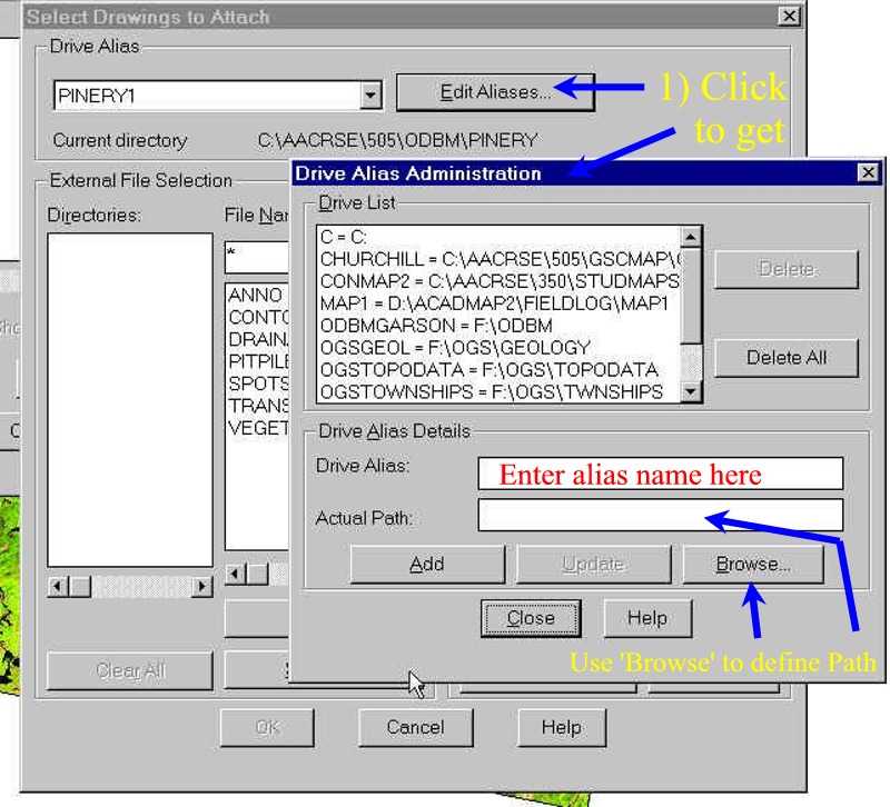
If an alias has not been defined, click the 'Create/Edit
Aliases' button (fourth button from the right) to fetch the 'Drive Alias
Administration' window. Provide a drive alias name in the requisite box,
and define the path in the 'Drive Alias Details' box (use BROWSE to define
the path) --> click Add followed by Close.
Alias Page
Select the alias name in the Drive
Alias box in the 'Select Drawing to Attach' window . A list of .DWG files
in the directory represented by the alias name will appear in the File
Name selection box -> click 5105150nad83, followed by ADD, and then OK
twice.
To plot the maps to the screen, make the selection
sequence:
Map -> Query -> Define query to call the
Query window.
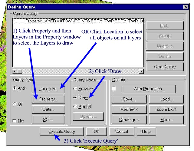
Query
window
Click 'Property', then the Layers button
followed by the Values button. In the drop-down selection list hold down
the CTRL key and select the following layers:
Building_to_Scale, Building_Symbolized,
Monument_Horizontal_Control, Rail_Line, River_Stream, Road_Centreline,
Shoreline, and Trail. Click OK twice.
Location
Condition window
Click the DRAW button in the Query Mode box ->
and the Execute Query button. Carry out a 'Zoom (z) Extents (e)' to display
the image.
Repeat for tile 5105140nad83.
c) Scanning a base map or aerial photograph
Image
File Size
An aerial photograph is about 9 inches by 9 inches size, and scanned at
a resolution of 600 dpi the photograph is composed of about 29 million
pixels representing a .tif file size of about 27 Mb. If viewed in
Microsoft Photoeditor the image size is about 5100 x 5400 pixels.
If this image is saved as a greyscale .jpg image at 80% quality the file
size will be reduced to 5.5 Mb. Such an image can be zoomed to about 400%
before excessive pixelation takes place. After gamma corection the file
size can be reduced to about 3.2 Mb. The resolution will be sufficient
to resolve a car on the highway, but not the driver. It should be possible
therefore to identify an outcrop a few square metres in size.
Scanning
procedure
Click Start ->
Programs
-> HP Desckscan II ->
HP
Deskscan II
In the Desk Scan II window select Edit
-> Preferences
and click the 'Better Illumination'
button in 'Image Quality'.
Click OK.
Click Custom
-> 'Preview Size'
and click and drag the bottom right corner of the white window in 'Window
Size' down to the bottom right to its maximum size. Click OK.
Click Custom
-> 'Print Path'
select 'screen'
in the right hand drop down selection list.
If the scanned image is a paper basemap
set the values in the Horizontal and Vertical 'Drawings
and Half-Tones' dpi box to 300. Click OK.
In the DeskScan II window, the scan 'Type'
should be selected as 'Sharp B. and W. Drawing',
whereas the scan 'Path'
should show as 'Custom'.
If the scanned image is a photograph
set the values in the Horizontal and Vertical 'Photos' dpi box to 600.
Click OK. In the DeskScan II window, the scan 'Type'
should be selected as 'Sharp Millions of Colours',
whereas the scan 'Path'
should show as 'Custom'.
Click 'Preview'
to inititate the scan.
The scanning lamp will warm up and the scan will proceed.
Click and hold the left mouse point at a point on the image representing
the lower left corner of the area of the map to be scanned, and then 'drag'
the mouse to the top right corner of the area. Click the Zoom button to
get a better view of the selected area. Click the Final
button. You will be asked to supply a name for the file. Enter a name and
indicate the path to the folder in which the file is to be stored, and
then click OK. The photograph will be scanned as a .tif
file to the indicated folder.
If the image is a photograph, import the image into an image editor such
as Corel PhotoPaint or Microsoft PhotoEditor in order to lighten any overly
dark areas with a gamma correction. Save the image as a greyscale
.jpg image.
Attaching the scanned base map to the Autocad Virtual Image and resampling the attached image
To Attach the scanned base map (or airphoto
or magnetic or geological map) to the Autocad .dwg drawing file, first
make
the relevant layer (e.g. Photo12) current (see The
Layer and Line Type Property Window), secondly, estimate
approximately the coordinates of the lower left corner of the image, and,
finally, carry out the operation Map
-> Image -> Insert ->
In the 'Image Insert' window select the file to attach and click the OPEN
button.
In
the subsequent INSERT window,
click the Pick
button. A cursor in the form of a +
will appear on the screen with a small rectangle in the top right segment
of the +. Click the the lower left corner
of the rectangle already drawn to represent the airphot (the rectangle
on layer 'Photoboundary12', and drag the cursor up and to the left to enlarge
the rectangle to approximately the size of the image being attached. Click
the left mouse button followed by either the right mouse button or the
ENTER key. Click the OK button in the Insert
window that should now have reappeared on the screen. At this stage the
placement of the image does not have to be accurate. Use Tools
-> 'Display Order' -> 'Send
to back' to place the image layer behind the location layer.
[If using Autocad Map r 2,
use the sequence Insert (on the Toolbar)
-> 'Raster Image'. In the Raster
Image window click the Attach button, then in the resultant 'Attach
Image' window click the Browse
button and in the 'Attach
Image File' window select the .TIF image you wish to insert.
Click the Open button. This will return you
to the 'Attach Image' window. In the Image
Parameters section, enter a rough estimate of the location of the
bottom left hand corner of the airphoto in the 'At:'
data entry box, click the 'Specify on Screen'
button for the Scale Factor, specify the rotation angle as '0', and then
click OK. A rectangle representing the relative
dimensions of the image will appear on screen. Within the rectangle will
be a rubber band which when dragged will redefine the dimensions of the
rectangle. Drag the rubber band to create a rectangle that approximates
the area of the photo as estimated from the plotted locations, and click
the left mouse button to terminate.]
Rubber Sheeting
Using the Rubber Sheet facility of Autocad
Map, the next operation will calibrate the UTM grid locations on the scanned
base map with those plotted on the location layer e.g. Coordinatepoints12.
Note, the first point entered will be the coordinate locality on the image,
the second point will be the corresponding locality on the location layer.
[It is also possible to attach a georegistered Spot, Landsat, or Radarsat
(8 meter resolution) image to the drawing project, and use this image as
a template to rubber sheet the airphotos.] When rubber sheeting,
freeze
all objects that do not need to be reoriented. Also, lock
(but do not freeze) the layer containing the location points that you are
going to use as reference points, otherwise they may be moved as part of
the rubber sheeting reorientation.
To carry out the rubber sheet operation, first
toggle OSNAP Off by
double clicking the OSNAP
button on the tool bar at the bottom of the screen, and then run the sequence:
Map->'Map
Tools' -> 'Rubber
Sheet'. On the command line Autocad
will request that you input 'Base Point 1'. To zoom into the location
points while carrying out the rubber banding, enter
'z (apostrophe z) and window the area around the base point and
the reference location. Then click on the base point on the photograph,
turn OSNAP on, and then click the reference point. Do a 'z,
p sequence to zoom back out to extents, and a 'z
w to zoom down to the next base point, etc, etc. When you have finished
adding base points and are zoomed out, press the ENTER key. Choose the
Select option by entering 's' on the command line, press ENTER, and click
the edge of the image. The image will change shape according to the reference
data entered during the rubber sheeting.
Alternatively, if a scanned image is not
available, use a digitizing tablet to calibrate the photograph or geological
map, using the already plotted points as a template to provide the coordinate
values (no need to type in the values each time a calibration is carried
out).
Making
the scanned basemap transparent
Run
the sequence Map
->
Image -> Properties
->
select the image and
press ENTER -> click
select and click
on the background colour of the image ->click
the 'Enable Transparency' button ->click
OK. The background of the image should now
be transparent.
7) Now that the base map has
been registered and/or the digital basemap has been attached and queried,
the airphoto can now be scanned, attached,
and registered to the basemap.
Make the Glocationbasemap
layer current
and plot the reference locations using
Draw
->
Point -> 'Single
Point' -> with
OSNAP enabled click the relevant location on the base map.
Create a Glocationbasemapnames layer, make
it current, and using the Text command,
enter a descriptive name or the coordinate value of the point.
8) Attach and resample (Rubber band) the airphoto, using the relevant reference points on Glocationbasemap.
9) attach and resample the relevant portion of geological map OGS 2491, first creating a Glocation2491and a Glocation2491names layer.
Data
Layering
Once the base maps, geological maps,
and photographs have been registered, we then need to create a set of layers
for the geographical and geological information that is to be plotted or
accessed on the map:
Alines 2491
Geological boundaries
Alinestemp
temporary lines
Beds2491
trends of bedding taken from map 2491, and trend lines based on
all bedding orientations
Faults2491
faults taken from map 2491
Geolbruce2491
polygons for the Bruce Formation
Geolbruce2491fil
colour filled polygons for the Bruce Formation
Geolgabbro2491
polygons for the Nipissing diabase
Geolgabbro2491fil colour filled
polygons for the Nipissing Gabbro bodies
Geolpecors2491
polygons for the Pecors Fm
Geolpecors2491fil colour
filled polygons for the Pecors Fm.
Geolsuddiab2491
polygons for the Sudbury diabase
Geolsuddiab2491fil colour filled
polygons for the Sudbury diabase bodies
GeolMiss249
polygons for the Mississagi Fm
GeolMiss249fil
colour filled polygons for the Mississagi Fm.
ETC
Glakes2491
lakes
Grail2491
railroads
Groads2491
roads
Gwater2491
rivers and streams
ETC
Studentsstati
stati localities on student maps
Studentsstruct
oriented bedding symbols, data from student maps
Studbrucestud
Studbrucestudfil
ETC
Use the Autocad SKETCH or PL (polyline) functions to copy geological boundaries, faults, water bodies, etc, to the corresponding layer in Autocad Map (e.g. Geolgabbro2491 = gabbro unit on geology map 2491.)
To do this you will need to learn how to digitize map data in Autocad, either from a georegistered map image ('heads up'), or by using a digitizing tablet:
Drawing
in Autocad - http://instruct.uwo.ca/earth-sci/505/draw1.htm
Drawing
using the Fieldlog Database - http://instruct.uwo.ca/earth-sci/505/draw2.htm
Calibrating
the tablet - http://instruct.uwo.ca/earth-sci/505/draw3.htm
(If the objects you are
going to digitize are on maps of different scales, see:
http://instruct.uwo.ca/earth-sci/505/draw3.htm#IMPORTANT1
Plotting
Window the area you would like to output. Click
File -> Print.
In the 'Plot/Configuration' window note that
the 'Window' button in 'Additional Parameters' has been selected.
Click the MM button in 'Paper Size and orientation',
and in the 'Scale, Rotation and Origin' box enter 50 for 'Plotted MM' and
1000 for 'Drawing units', where '50' means millimetres and '1000' means
metres; make sure the 'Scaled to Fit' box is deselected (no tick);
In the 'Plot Preview' box click the Full button
and then click 'Preview'; a view of the image on the page should appear;
if the image is as it should be click ESc to return to the 'Plot/Configuration'
window, and click OK to print.
RETURN TO: