Lec 2: Reality,
Data
“Art
is a lie which makes us realize the truth” (Picasso)
Quote
from the Introduction to Part I of the book
Do you
want to understand Part I — on “Map Reading” and its 10 Chapters?
If
so, then read the Intro to Part I (pp. 17-18)
To
quote from Paragraph 2 on p. 18:
“Since
the exact duplication of a geographical setting is impossible, a map is
actually a metaphor. The map maker asks
the map reader to believe that an arrangement of points, lines, and areas on a
flat sheet of paper is equivalent to a multidimesional world in space and
time. For full meaning, the map reader
must go beyond the paper-and-ink representation to the real world referents of
the system.”
Is
this true?
Since
Chapter 1 is about The Environment to be Mapped
let’s
look at an environment and at a modern map of that environment
...
and assess the validity of the quoted assertion
Saline
Valley slideshow versus a “modern map viewing experience”
So
what’s the verdict?
Discussion
Today’s
Lecture
Geographic
Reality
Geographic
Data
Geographic
Reality
The
Physical (or “Material”) World
The
concept of a geographic feature
a
“geography as geometry” point of view
Feature hierarchy
Declarative
Object
physical
(eg. “bridge”)
conceptual
(“soil type”)
Relation
derived,
form/pattern, spatial arrangement (eg. “centroid”)
Procedural
Process (eg. “air mass flow”)
has
temporal component
Form
Discrete
Dispersed/Discontinuous
features
Continuous
phenomena
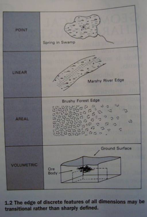
Discrete
(Figs 1.1., 1.2)
Fig
1.1.
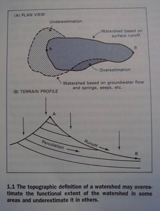
Fig
1.2
Dispersed/Discontinuous
features
E.g.:
Rock
Outcrops
Park
Forest
Houses
in a village
and
other “salt or pepper” distributions
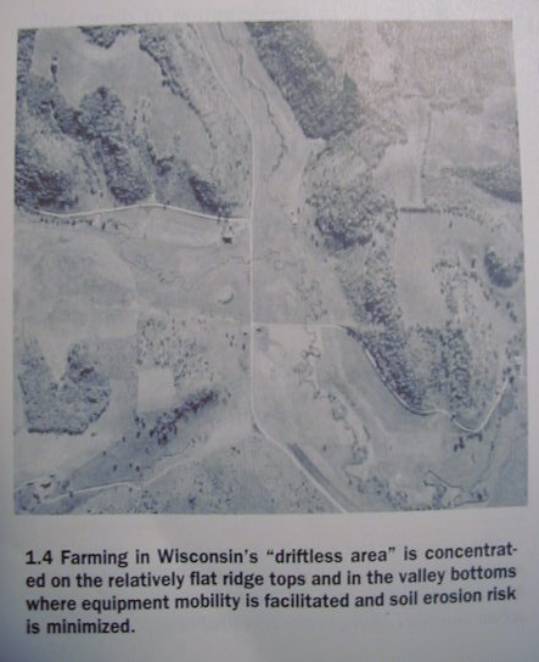
Continuous
phenomena (Figs 1.4 - 1.7)
Mosaic,
Stepped, or Smooth surfaces
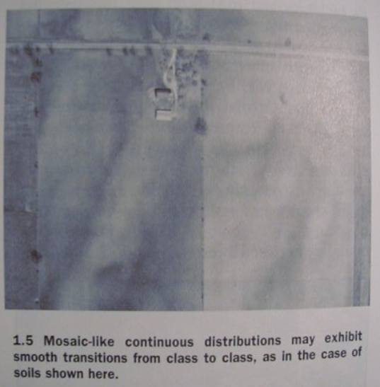
Mosaic
surfaces
w/distinct
border (rare)
w/continuous
transitional boundaries (more common)
Fig
1.4
Fig
1.5
Stepped
surfaces
terraces
nature
tends to smooth gradual transitions
Fig
1.6
Smooth
surfaces
eg.
elevation
environmental
gradients
Dimensionality
of Environment
Fig
1.9
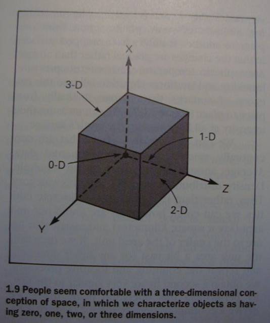
Quote
p. 26 para 2
“We
learn early that objects have three dimensions: length, width, and height. If all three dimensions are 0, we have a
0-dimesional (point) object. If two
dimensions are 0, we have a one-dimesional (linear) feature. If only one dimesion is 0, we have a
two-dimensional (area) feature. If an
objects exhibits all three dimensions, we have a three-dimensional solid
(volumetric) feature. In geographical
terms, length and width become area or region, and height becomes elevation or
magnitude.”
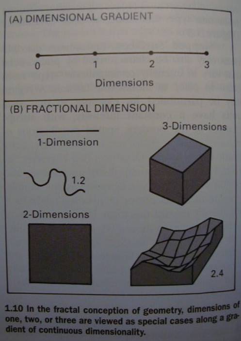
dimensions
0-3D
fractals
T
Fig
1.10
Environmental
Change
spatio-temporal
context
static
vs. dynamic feature
depends on/relative to a temporal scale
The
Nature of Time
T
is relative
natural time
biological time
clock or calendar time
...and their importance in Aviation
Enviromental
Temporality
Change of Environmental Features
change in State
change in Position
rate
of change
Quote
(pp. 28-29)
“Things that happen too fast we miss. We may also miss changes that happen too
slowly. This is a common problem when observing our environment. Pollution creeps into lakes and streams,
fields are eroded, and living things become extinct, all before we realize
what’s happening. We humans are adept at ignoring the passage of time. That’s
why high-school reunions are so shocking.
What a blow to discover that while we haven’t aged, all our classmates
have!”
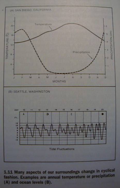
Fig
1.11
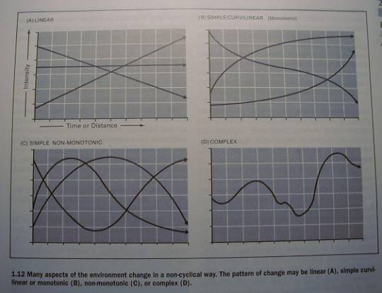
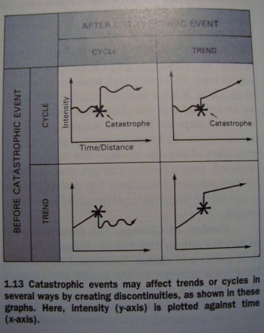
Pattern of change
cycles
trends
catastrophes
Fig.
1.12
Fig
1.13
Movement through space — of
discrete
point features
linear
areal
volumetric
Break
Representing
the Real World
Representing
a student in the class
Call for a volunteer ...
PinPoint
= 2 310
Low-Res
Computer Monitor 640x480 = 307 200
We
will refer to this experiment as the lecture unravels
Representing
the whole class
List
Name,
Student Number, Program, Year
Students
as Geographic Features...
Snapshots
with
Name (Last, First)
Geographic
Data
The
issue of data quality
(a
bit like cars, drugs, cooking recipe ingredients)
Aspects
of information gathering which influence mapped data
the
method used to gather data
the
way the data are structured
the
nature of the quantification achieved
the
data inventory scheme
the
derivation of statistical summary measures from raw data values
Acquisition
Method
Ground
Survey
horizontal
and vertical measurements
Horizontal
measurements
horizontal
reference datums (Fig. 2.1)
ellipsoids
Fig.
2.1
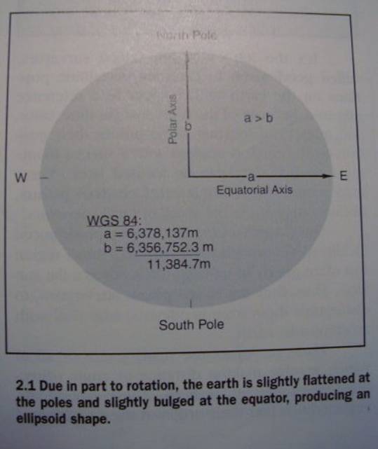
Fig.
2.2a
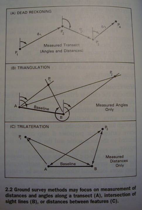
Dead
Reckoning
Triangulation
Trilateration
Fig.
2.2
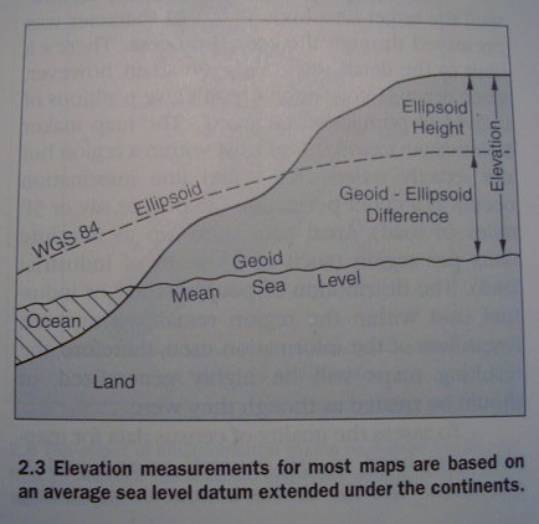
Vertical
measurements
elevation
vertical
reference datums
mean
sea level (MSL)
geoid
geoid-ellipsoid
differences (Fig. 2.3)
Fig.
2.3
Global
Positioning System (GPS)
Modern
survey measurements
Self-Study
sub-units:
Census
Remote
Sensing
Compilation
Data
Model
Object-Oriented
Model
(Vector GIS, CAD)
Location
Oriented Model
(Grid-based, Raster GIS, cell, pixel, matrix, array,
image)
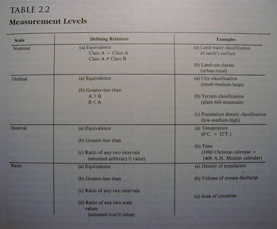
Measurement
Level
Table
2.2
Inventory
Scheme
Population
Counts
errors
instrumental
methodological
human
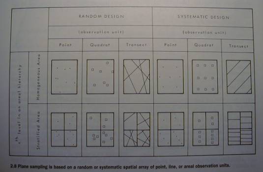
Spatial
Samples
Fig.
2.8
Spatial
Prediction
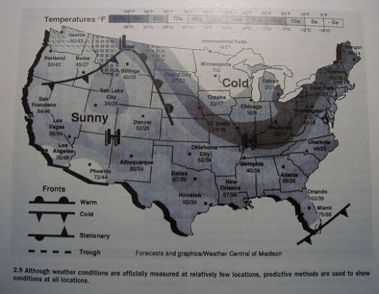
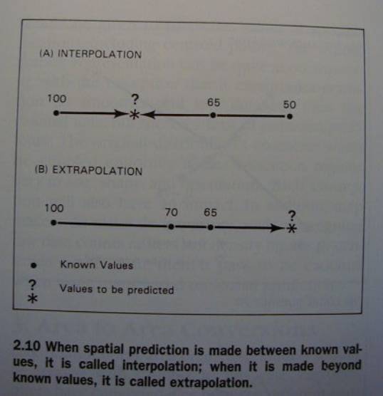
Point
to Point Conversions (Figs 2.9 and 2.10)
Interplolation
Extrapolation
Fig
2.9
Fig
2.10
Also
discussed are:
Area
to Point Conversion (eg. Population Density sample areas)
Area
to Area Conversion (eg. Zonal Transformation)
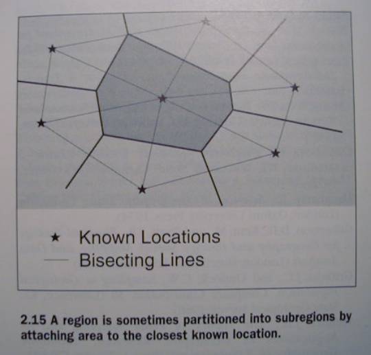
Point
to Area Conversion (partitioning space, eg. Fig. 2.15 via Thiessen Polygons,
Voronoi Diagrams)
Fig
2.15
Derived
Values
values
derived from transforming data
logical,
arithmetic, statistical transformations
statistical
summarize values in the form of a statistic representing a
typical value
characterize the variation within an existing set of
values
summarize values in the form of a statistic representing
an atypical value
(e.g.
extremes, outliers, anomalies)
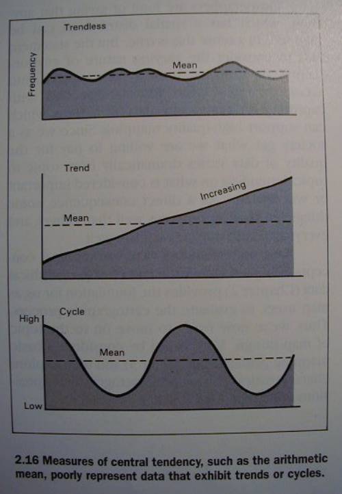
Fig.
2.16