Lec 7: Spatial Primitives: Direction and Distance

Sphere of Distance (Haul Cost Analysis)

Announcements

The Readings for Today’s Lecture were:

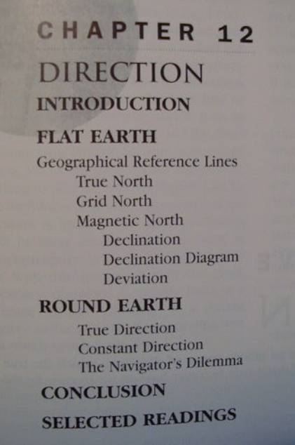
Ch. 12: Direction

Ch. 13 Distance

Assignments:

Lab for Assignment No. 3

The material in the second part of the term is moving

from background basics

towards Navigation

Extensive land navigation last week

using the best students for winter night navigating of dark wet twisty country lanes...

astronaut nav story

Comments or Questions?

Today’s Lecture:

Direction

Distance

Direction

Spatial Relations

Give me Examples

Here is my partial list:

...for instance:

distance

direction

proximity (adjacency)

segregation (insularity), aggregation

contiguity (continuity), discontinuity (disjointness)

containment (inclusion), complete, partial

What are the two most basic (“primitive”) spatial relations?

Distance and Direction

and the text devotes a whole chapter to each

Direction

TOC

Key issues concerning Direction

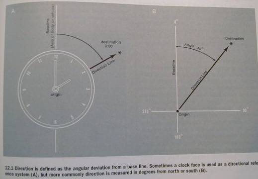
Def.: The angular deviation from a base line

Egocentric vs. Geocentric base line.

Fig. 12.1

Geographic Reference Lines

use North-South as the base line

problem is: there are three norths!

True (or Geographical) North

refers to the North Pole

meridians of longitude

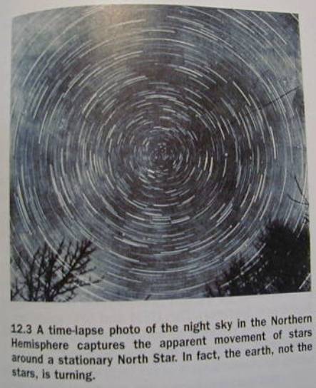
North Star (Polaris)- about 1 degree off

Fig. 12.2

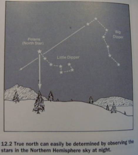
Fig. 12.3

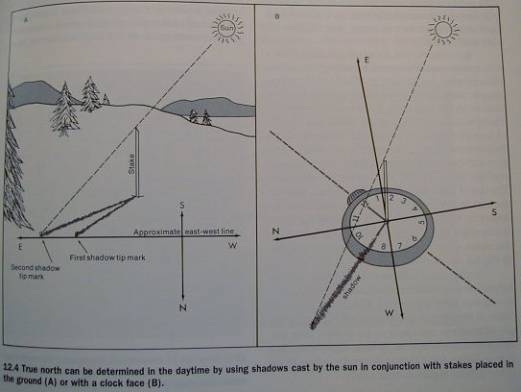
Sun - Fig 12.4

Artificial satellites

GPS

Grid North

Fig. 12.5

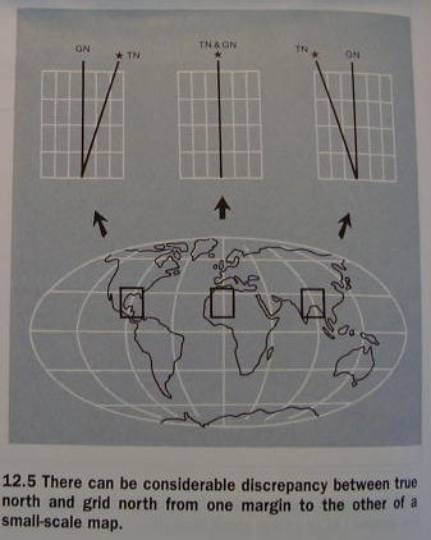
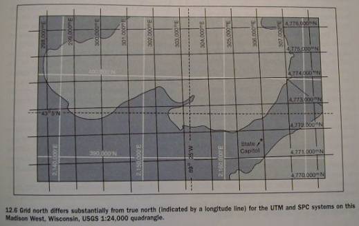
Fig 12.6

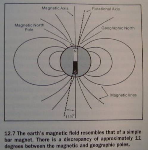
Magnetic North

Magnetic Compass

Geomagnetic field - Fig. 12.7

GPS Compass

Declination

Grid Declination - the angular difference between a grid line and true north

Magnetic Declination - the angular difference between true north and magnetic north

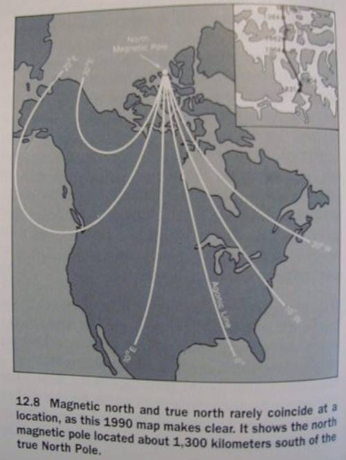
How much is the magnetic declination in Blue mountain Lake (Adirondack Mountains, New York)?

Fig. 12.8

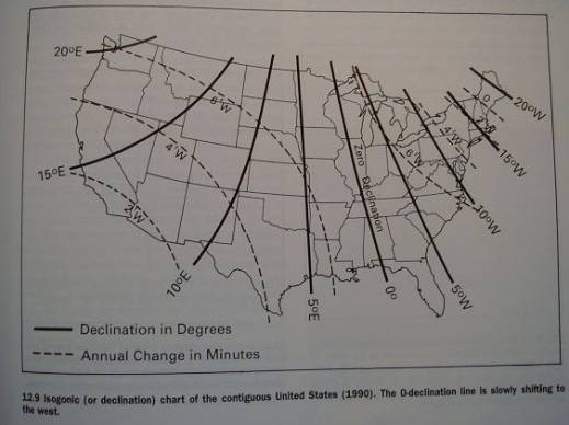
Maps with isogonic lines

Fig. 12.9

Polar bears aren’t the only things that wander in the north

so’s the magnetic north!...

chemical magnetism

and proof for continental drift

Navigation problems due to Declination are compounded with distance

thus aeronautical and nautical charts, and large-scale maps designed to be used in the field provide a:

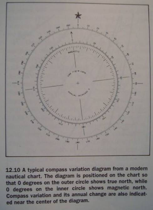
Compass Variation Diagram

Fig 12.10

Declination Diagrams

Are provided with the standard USGS Topo Quad Series

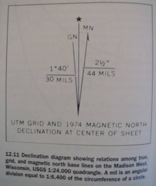
The declination is for the center of the map, and its accuracy decays toward the map edges

Fig 12.11

Tips for using very small declination diagrams

Use a straight-edge to extend the lines, then measure

Make sure the graphic angles are correct (rather than schematic)

otherwise redraw the lines with a protractor using the numerical annotation

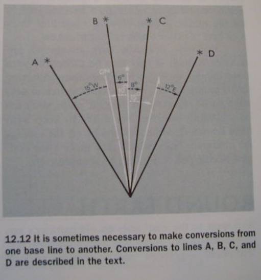
Conversions

from one base line to another

made by simply adding or subtracting

but this can be confusing

tip: solve it graphically

Problem: What should you set the Auto Pilot Bearing (Compass Direction) to in order to get:

from Lake Durant (el. 1830’) to Mount Marci (el. 5344’)

Map (True North) bearing from Lake Durant is 49 Degrees.

Declination is 14 Degrees W (cf. Fig. 12.9)

Compass Azimuth should be set to: ....?

Answer: 63 degrees

*Sketch *

Note:

our example problem is similar

to the example in Fig 12.12 for converting direction line D to a true direction value

Fig 12.12

Deviation

Declination doesn’t tell the whole story:

“Not only does the compass needle rarely point to true north—it often doesn’t even point to magnetic north !

This discrepancy is called deviation,

and is due to regional or local magnetic irregulariries

systematic, stable irregularities may be shown on the isogonic declination maps,

however, local sporadic irregularities won’t, eg. power lines, ore bodies, and thunderstorms

monitor the behavior of your compass, watch out for erratic needle behavior...

Round Earth

“Determining direction on a round earth, as every ship and plane pilot knows, is a far different matter than flat-world direction finding”.

The simple definition of direction no longer holds when the earth roundness is factored in

Two ways to interpret direction on a spherical earth:

true azimuth - shortest distance route betweeen two points

constant azimuth

True Direction

a direction line which forms a full circle is called a true azimuth

great circle is defined as:

all true azimuths other that east-west (Q:Why? A: ”Eq...”)

and all true azimuths other than those originating from a point on the equator

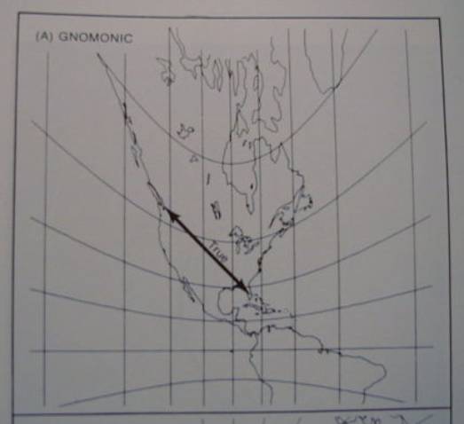
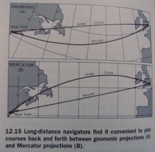
great circles are the shortest possible routes between two points on earth

only the gnomonic projection

portrays great circles as straight lines

Fig 12.13a

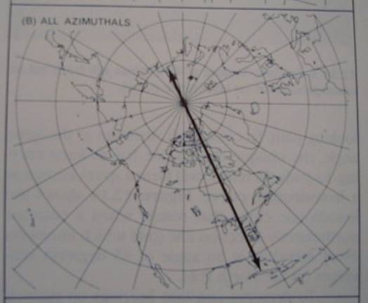
all azimuthal projections

can show more than a hemisphere

but can only correctly show true azimuths that pass through their central points

Navigators need maps they can keep using as their course changes from a planned route

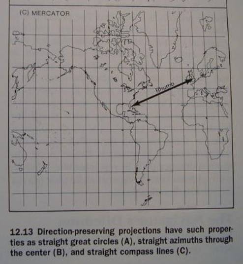
Fig 12.13b

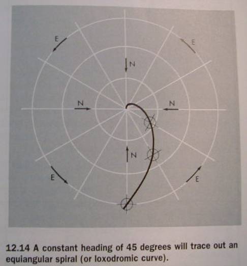
Constant Direction

“A direction line which is extended so that it crosses each meridian at the same angle is called a constant azimuth (or a rhumb or loxodrome).”

thereful extremely useful for navigators

the paths are actually curving in a spiral known as a loxodronic curve

Fig 12.14

The Mercator projection

solves the problem of providing a map where

constant directions are straight lines,

hence extremely useful for global navigation

Fig 12.13c

The Navigator’s Dilema

What is it?

How solved?

A beautiful example of problem solving in a ‘trade-off problem’ context

see p. 256 in the textbook.

Fig 12.15

Break

Distance

TOC

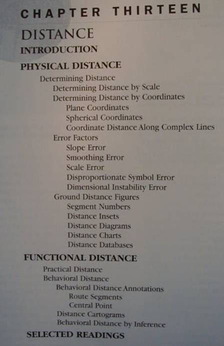
Physical Distance

standard units of measurement

(Statute) Mile (5280 feet)

Geographical Mile

International Nautical Mile

International Nautical Mile (6076.1 feet or 1852 meters)

standard unit of distance in water and air navigation

and the basis for calculating speed in knots

represents 1 minute of a great circle of a perfect sphere whose area is equal to the area of the earth

English system units versus Metric system units

Metric is decimal based - convenient for calculations

Conversions are necessary (Tables E3 and E4)

GPS systems do both

Determining Distance

Maps are useful for determining distance

By scale or using coordinate Pythagorean algebra (the Distance Theorem)

Determining Distance by Scale

use of the representation fraction (RF)

use of the graphic scale

Fig. 13.1

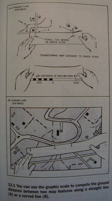
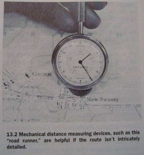
use of distance measurers

“road runner”

Opisometer - Fi g. 13.2

Determining Distance by Coordinates

lends itself particularly well to automation

computer software (eg. MFworks)

GPS

Plane Coordinates

for relatively small areas of the earth, eg. covered by a UTM map sheet

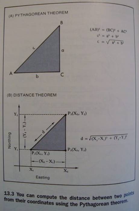
is an adaptation of the Pythagorean Theorem

see (and learn) the equation

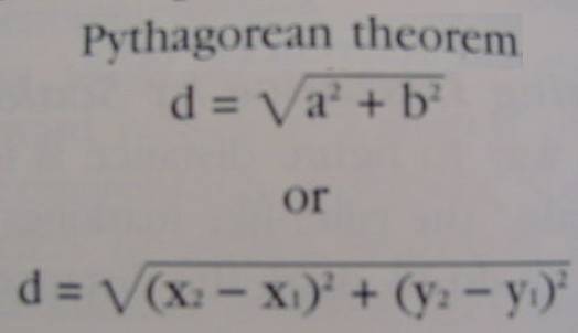
Fig 13.3

Example from the text:

Fig. 13.4

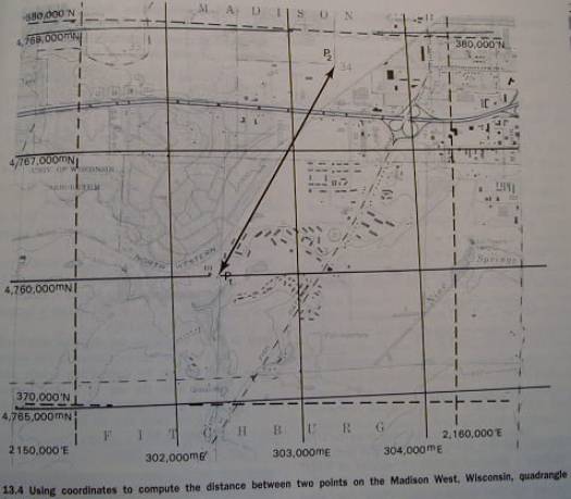
This example:

walks you through the calculations (using both SPC and UTM)

comes up with a distance 6604 feet (UTM)

and also compares it to (graphic) map scale method ( which came to 6600 feet)

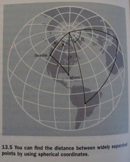
Spherical Coordinates

when the distances are considerable on a global scale

is based on the Geographical Grid and its angular properties

...along with the basic Trigonometric function:

cos a = (cos b) (cos c) + (sin b) (sin c) (cos A)

Fig. 13.5

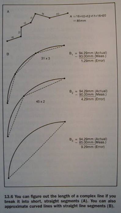
Coordinate Distance Along Complex Lines

for complex lines or for curved lines

break the line into short straight segments (fine-coarse tradeoff in effort vs. accuracy)

then follow the same procedure to measure the distance for each segment (“leg”),

and finally: add them up

Fig. 13.6

Error Factors

External error factors

external to the map

Internal error factors (and how to deal with them)

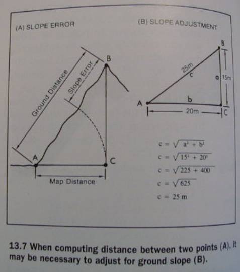
Slope Error

Fig 13.7

Smoothing Error

due to map scale vs. reality

mitigate by using large-scale maps

problem: variable smoothing (within a map)

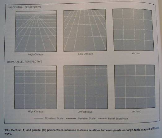
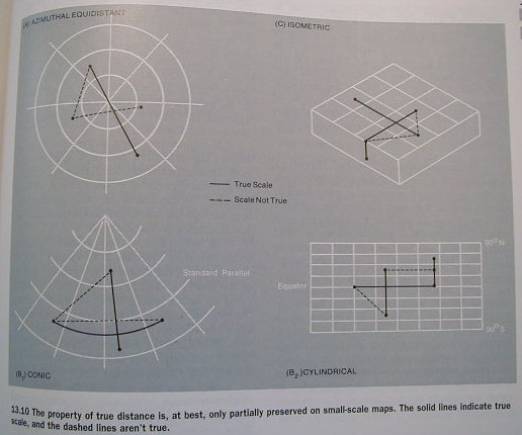
Scale Error

Scale varies in the map in central perspective maps (not so in parallel perspective maps)

Scale varies in oblique vs orthogonal maps

Fig 13.9

Azimuthal equidistant maps offer partial solutions for small-scale maps

Fig 13.10

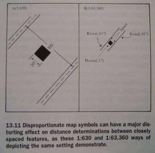
Disproportionate Symbol Error

Fig 13.11

Dimensional Instability Error

for example paper shrinkage and expansion (non-uniform)

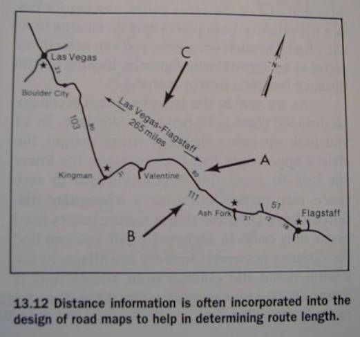
Ground Distance Figures

Some distances have been measured on the ground and recorded on maps

Segment Numbers and Distance Insets

Fig. 13.12

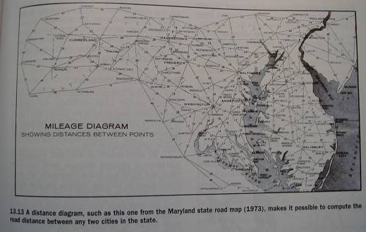
Distance Diagrams

where routes between features are abstracted to distance-annotated straight lines

Fig. 13.13

Distance Charts

rectangular tables and triangular charts

Fig. 13.14

Distance Databases

and accompanying software

including on the internet

Functional Distance

Practical Distance

differ due to

events (eg. missed turn)

constraints (eg. detours)

Behavioral Distance

Behavioral Distance Annotations

Fig. 13.15

Behavioral Distance by Inference

eg. our choice of route in London at certain times of the day/year changes

the route may be modified by applying our experience

‘til next week!