Lab Two: Probability Distributions
Objectives:
To learn when and how to calculate probabilities from the Binomial, Poisson and Normal distributions, using "hand" techniques (ie. calculator and tables).
Binomial:

where n is the number of events; p is the probability of the "given" outcome; q = 1—p; and X is the number of times the "given" outcome occurs within the n trials.
When a coin is flipped, the outcome is either a head or a tail; when a magician guesses the card selected from a deck, the magician can either be correct or incorrect; when a baby is born, the baby is either born in the month of March or is not. In each of these examples, an event has two mutually exclusive possible outcomes. For convenience, one of the outcomes can be labeled "success" and the other outcome "failure." If an event occurs N times (for example, a coin is flipped N times), then the binomial distribution can be used to determine the probability of obtaining exactly r successes in the N outcomes. The binomial probability for obtaining r successes in N trials is:
where P(r) is the probability of exactly r successes, N is the number of
events, and p is the probability of success on any one trial. This formula
assumes that the events:
(a) are dichotomous (fall into only two categories)
(b) are mutually exclusive
(c) are independent and
(d) are randomly selected
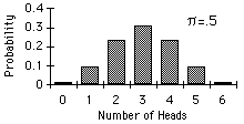
Consider this simple application of the binomial distribution: What is the probability of obtaining exactly 3 heads if a fair coin is flipped 6 times? For this problem, N =6, r=3, and p = .5.
Therefore,
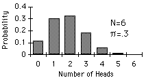
Two binomial distributions are shown below. Notice that for p = .5, the distribution is symmetric whereas for p = .3, the distribution has a positive skew.


Often the cumulative form of the binomial distribution is used. To determine
the probability of obtaining 3 or more successes with n=6 and p = .3, you
compute P(3) + P(4) + P(5) + P(6). This can also be written as:
and is equal to .1852 + .0595 + .0102 + .0007 = .2556. The binomial
distribution can be approximated by a normal
distribution (click here
to see how). Click here
for an interactive demonstration of the normal approximation to the binomial.
Binomial discussion and example taken from: http://davidmlane.com/hyperstat/A2301.html
of Rice Virtual Lab in Statistics at http://www.ruf.rice.edu/%7Elane/rvls.html
Poisson:

where 8 is the mean occurrence per unit of time, and X is the number of occurrences and e = 2.7183 .
Determining the probability of a rare event
Let us assume that the probability of finding an ancient artifact is described by a Poisson distribution with a mean of 2.3 finds per 10000 tries. What is the probability of observing a local retrieval rate of 6 artifacts per 10000 tries (assuming that nothing is acting to increase the rate)?
|
P(6) = e-2.3 2.36 / 6! P(6) = 0.1003 * 148.04 / 720 P(6) = 0.021 or 2.1% |
Important Normally we would rephrase the question slightly. If = 2.3 what is the probability of observing at least 6 deaths per 1000 rather than exactly 6 deaths per 10000? In other words we need to find P(6+) rather than P(6). By rephrasing the question we are saying that we wish to know the probability of occurrence of any event with the same or lesser probability. There is an important distinction between the probability of exactly 6 events and the probability of 6 or more events.
In order to find P(6+) we could calculate
1-[P(0)+P(1)+P(2)+P(3)+P(4)+P(5)]
or more simply look up P(6+) in tables). P(6+) = 0.03 or 3%
Normal distribution
Normal distributions are a family of distributions that have the same general shape. They are symmetric with scores more concentrated in the middle than in the tails. Normal distributions are sometimes described as bell shaped. Examples of normal distributions are shown to the right. Notice that they differ in how spread out they are. The area under each curve is the same. The height of a normal distribution can be specified mathematically in terms of two parameters: the mean (m) and the standard deviation (s).
The standard normal distribution is a normal distribution with a mean of 0
and a standard deviation of 1. Normal distributions can be transformed to
standard normal distributions by the formula:![]()
where X is a score from the original normal distribution, m is the mean of the original normal distribution, and s is the standard deviation of original normal distribution. The standard normal distribution is sometimes called the z distribution. A z score always reflects the number of standard deviations above or below the mean a particular score is. For instance, if a person scored a 70 on a test with a mean of 50 and a standard deviation of 10, then they scored 2 standard deviations above the mean. Converting the test scores to z scores, an X of 70 would be:
![]()
So, a z score of 2 means the original score was 2 standard deviations above the mean. Note that the z distribution will only be a normal distribution if the original distribution (X) is normal.
Applying the formula ![]()
will always produce a transformed variable with a mean of zero and a standard deviation of one. However, the shape of the distribution will not be affected by the transformation. If X is not normal then the transformed distribution will not be normal either. One important use of the standard normal distribution is for converting between scores from a normal distribution and percentile ranks.
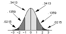
Areas under portions of the standard normal distribution are shown to the
right. About .68 (.34 + .34) of the distribution is between -1 and 1 while about
.96 of the distribution is between -2 and 2.
If the mean and standard deviation of a normal distribution are known, it is relatively easy to figure out the percentile rank of a person obtaining a specific score. To be more concrete, assume a test in Introductory Psychology is normally distributed with a mean of 80 and a standard deviation of 5. What is the percentile rank of a person who received a score of 70 on the test? Mathematical statisticians have developed ways of determining the proportion of a distribution that is below a given number of standard deviations from the mean. They have shown that only 2.3% of the population will be less than or equal to a score two standard deviations below the mean.. In terms of the Introductory Psychology test example, this means that a person scoring 70 would be in the 2.3rd percentile.
This graph shows the distribution of scores on the test. The shaded area is 2.3% of the total area. The proportion of the area below 70 is equal to the proportion of the scores below 70.
Similarly, the proportion of the area below 75 is the same as the proportion of scores below 75.
Mathematical statisticians have determined that 15.9% of the scores in a normal distribution are lower than a score 1 standard deviation below the mean. Since 75 is 1 standard deviation below the mean, the proportion of the scores below 75 is .159. Therefore, a person scoring 75 would have a percentile rank score of 15.9.
The table gives the proportion of the scores below various values of z. z is
computed with the formula
where z is the number of standard deviations above the mean (m) the score X
is. The standard deviation is s. When z is negative it means that X is below the
mean. Thus, a z of -2 means that X is -2 standard deviations above the mean
which is the same thing as being +2 standard deviations below the mean. To take
another example, what is the percentile rank of a person receiving a score of 90
on the test?
The graph shows that most people scored below 90.
Since 90 is 2 standard deviations above the mean [z = (90 - 80)/5 = 2] it can be determined from the table that a z score of 2 is equivalent to the 97.7th percentile: The proportion of people scoring below 90 is thus .977
What score on the Introductory Psychology test would it have taken to be in the 75th percentile?
(Remember the test has a mean of 80 and a standard deviation of 5.) The answer is computed by reversing the steps in the previous problems. First, determine how many standard deviations above the mean one would have to be to be in the 75th percentile. This can be found by using a z table and finding the z associated with .75. The value of z is .674. Thus, one must be .674 standard deviations above the mean to be in the 75th percentile. Since the standard deviation is 5, one must be (5)(.674) = 3.37 points above the mean. Since the mean is 80, a score of 80 + 3.37 = 83.37 is necessary. Rounding off, a score of 83 is needed to be in the 75th percentile.
Since ,
a little algebra demonstrates that X = m+ z s. For the present example, X = 80 + (.674)(5) = 83.37 as just shown.
If a test is normally distributed with a mean of 60 and a standard deviation
of 10, what proportion of the scores are above 85? This problem is very similar
to figuring out the percentile rank of a person scoring 85. The first step is to
figure out the proportion of scores less than or equal to 85. This is done by
figuring out how many standard deviations above the mean 85 is. Since 85 is
85-60
= 25 points above the mean and since the standard deviation is 10, a score of 85
is 25/10 = 2.5 standard deviations above the mean. Or, in terms of the formula,
A z table can be used to calculate that .9938 of the scores are less than or equal to a score 2.5 standard deviations above the mean. It follows that only 1-.9938 = .0062 of the scores are above a score 2.5 standard deviations above the mean. Therefore, only .0062 of the scores are above 85
Suppose you wanted to know the proportion of students receiving scores
between 70 and 80. The approach is to figure out the proportion of students
scoring below 80 and the proportion below 70. The difference between the two
proportions is the proportion scoring between 70 and 80. First, the calculation
of the proportion below 80. Since 80 is 20 points above the mean and the
standard deviation is 10, 80 is 2 standard deviations above the mean.
A z table can be used to determine that .9772 of the scores are below a score
2 standard deviations above the mean.
To calculate the proportion below 70,
A z table can be used to determine that the proportion of scores less than 1
standard deviation above the mean is .8413. So, if .1587 of the scores are above
70 and .0228 are above 80, then .1587 -.0228 = .1359 are between 70 and 80.
Assume a test is normally distributed with a mean of 100 and a standard deviation of 15. What proportion of the scores would be between 85 and 105? The solution to this problem is similar to the solution to the last one. The first step is to calculate the proportion of scores below 85. Next, calculate the proportion of scores below 105. Finally, subtract the first result from the second to find the proportion scoring between 85 and 105.
Begin by calculating the proportion below 85. 85 is one standard deviation below the mean:
Using a Z table with the value of -1 for z, the area below -1 (or 85 in terms of the raw scores) is .1587.
Doing the same thing for 105,
A Z table shows that the proportion scoring below .333 (105 in raw scores) is .6304. The difference is .6304 - .1587 = .4714. So .4714 of the scores are between 85 and 105.
All of this material on the normal distribution and the calculation of areas under the curve are taken from : http://davidmlane.com/hyperstat/normal_distribution.html. The above text is provided as a convenience for you.
Some of the material and the interlink links have been edited out. I strongly encourage you to go to the Rice Virtual Lab in Statistics at http://www.ruf.rice.edu/%7Elane/rvls.html to look at the original pages.
For this exercise hand in written answers to the questions below.
Questions - Part I: Probability (80 marks)
1. An insurance company is examining the seismicity of an area to calculate premium levels on earthquake insurance. Over the past 50 years, 5 events powerful enough to inflict structural damage have occurred. What is the probability that there will be more than six such events over the next 40 years? [HINT: P(X) > 6) = 1 - (P(0) + P(1) + P(2) + P(3) + P(4) + P(5) + P(6))]
2. A city planner claims that 20 percent of all apartment dwellers move from their apartments within one year of taking up residence. In a given area, 15 apartment dwellers, who have just given notice to their landlords, are to be interviewed. What is the probability that 10 out of the 15 have been in residence for more than one year?
3. Geothermal prospecting in an area 20 km by 10 km reveals 18 exploitable sources, scattered randomly across the area. Using an appropriate probability model, calculate the chances of finding one or fewer sources in any given square kilometre quadrat.
4. A well known beer company is promoting a brand of beer by holding blind taste tests on two beer recipes: "X" and "Y3". The recipe preferred by most will be chosen as the brand recipe. If the chances of choosing either recipe are equal (ie .5 each), what is the probability that exactly 7 people out of 10 will choose "X"? What is the probability that at least 7 people out of 10 will choose "X"?
5. Past weather observations at a given station indicate that the maximum temperature on a given date averages 15°C, with a standard deviation of 3°C. Assuming that the data are normally distributed:
(a) What is the probability that a maximum temperature in excess of 20°C will occur?
(b) What is the probability that the maximum temperature will lie between 13.5 and 16.5 degrees?
6. The Geograd Union has a committee of 12 people. In how many ways can they choose:
a) a chairperson, a vice-chairperson, a secretary and a treasurer, assuming a person cannot hold more than one position? b) a subcommittee of 4 people?
7. An instructor randomly selected 1000 students to determine the relationship between grades and class attendance. The data obtained is found in the table below. Compute each of the following probabilities using the empirical approach.
| percentage of classes attended | |||||
| Grade | over 90% | 70% to 90% | 50% to 69.9% | 10% to 49.9% | less than 10% |
| A | 69 | 62 | 53 | 35 | 1 |
| B | 94 | 93 | 67 | 40 | 6 |
| C | 82 | 68 | 32 | 14 | 4 |
| D | 38 | 32 | 20 | 7 | 3 |
| F | 23 | 30 | 35 | 28 | 64 |
a) the probability of getting a A when attending less than 10% b) the probability of attending 50% to 69.9% of the time and receiving a B c) the probability of receiving an A.
8. The number of arrivals to a isolated border crossing is found to be 250 arrivals over 100 days. On one particular day what is the probability that there will no one crossing the border at that station? What's the probability of only one arrival? What's the probably of more than 4 arrivals?
To be completed in class: (20 marks)
1. Shuffle a deck of playing cards and draw 1 card. Repeat at least 50 times. Determine an estimate for the probability of drawing an ace from a deck of 52 playing cards. Is your answer consistent with what you would have expected to have happened?
2. Shuffle a deck of playing cards and deal a hand of 5 cards. Record whether all are red. Repeat this experiment at least 30 times and determine the experimental probability of dealing a hand of red cards.