|
|
|
|
One way ANOVA (the F ratio test) it is the standard parametric test of difference between 3 or more samples, it is the parametric equivalent of the Kruskal-Wallis test H0= :1=:2=:3=:k the population means are all equalso that if just one is different, we will reject H0 we expect that the sample means will be different, question is, are they significantly different from each other H0: differences are not significant - differences between sample means have been generated in a random sampling process H1: differences are significant - sample means likely to have come from different population means assumptions 1) data must be at the interval/ratio level 2) sample data must be drawn from a normally distributed population 3) sample data must be drawn from independent random samples 4) populations have the same/similar variances - homoscedasticity assumption from which the samples are drawn ANOVA examines differences in means by looking at estimates of variances essentially ANOVA poses the following partition of a data value observation=overall mean + deviation of group mean from overall mean + deviation of observation from group mean the overall mean is a constant to all observations deviation of the group mean from the overall mean is taken to represent the effect of belonging to a particular group deviation from the group mean is taken to represent the effect of all other variables other than the group variable examples: consider the numbers below as constituting One data set example 1:
Much of the variation is within each row, it is difficult to tell if the means are significantly different as stated before, the variability in all observations can be divided into 3 parts 1) variations due to differences within rows 2) variations due to differences between rows 3) variations due to sampling errors example 2;
much of the variation is between each row, it is easy to tell if the means are significantly different [note: 1 way ANOVA does not need equal numbers of observations in each row]
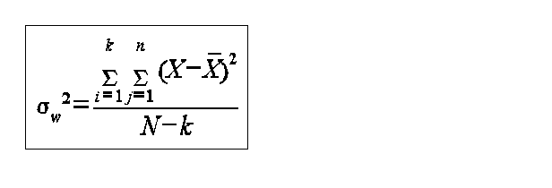
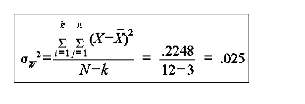
in example 1: between row variation is small compared to row variation, therefore F will be small large values of F indicate difference conclude there is no significant difference between means in example 2: between row variation is large compared to within row variation, therefore, F will be large conclude there is a significant difference the first step in ANOVA is to make two estimates of the variance of the hypothesized common population 1) the within samples variance estimate 2) the between samples variance estimate the within sample variance estimate is
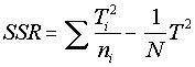
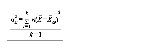
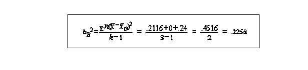
k - is the number of sample N - total number of individuals in all samples X bar - is the mean the between samples variance estimate is
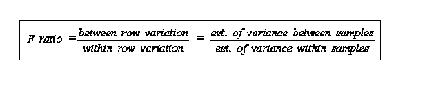
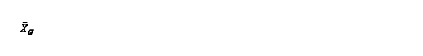
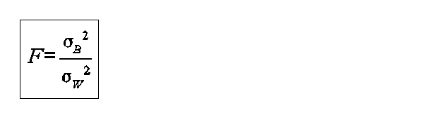
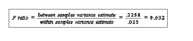
is the grand mean having calculated 2 estimates of the population variance how probable is it that 2 values are estimates of the same population variance to answer this we use the statistic known as the F ratio
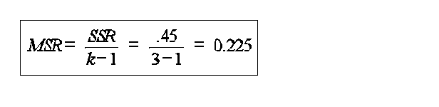
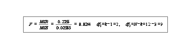
significance: critical values are available from tables df are calculated as 1) for the between sample variance estimate they are the number of sample means minus 1 (k-1) 2) for the within sample variance they are the total number of individuals in the data minus the number of samples (N-k) since the calculations are somewhat complicated it should be done in a table example Test winning times for the men�s Olympic 100 meter dash over several time periods
source: Chatterjee, S. and Chatterjee, S. (1982) �New lamps for old: an exploratory analysis of running times in Olympic Games�, Applied statistics, 31, 14-22. H0: There is no significant difference in winning times. The difference in means have been generated in a random sampling process H1: There are significant differences in winning times. Given observed differences in sample means, it is likely they have been drawn from different populations. Confidence at "=0.01, 99% confident from different population example table
calculation of between samples variance estimate
analysis of variance table
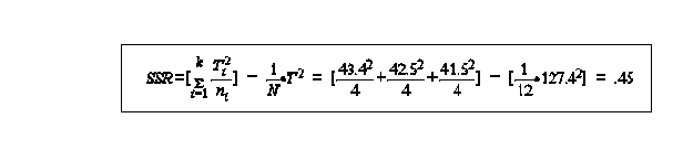
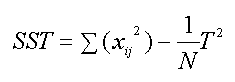
critical value=8.02, page 277 in text, "=.01 therefore we reject the null hypothesis computational formula one problem in using these formulas, however, is that if the means are approximated, the multiple subtractions compound rounding errors. To get around this, the formulas can rewritten as
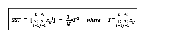
N=total number of observations T is the total sum of observations it can be shown that
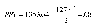
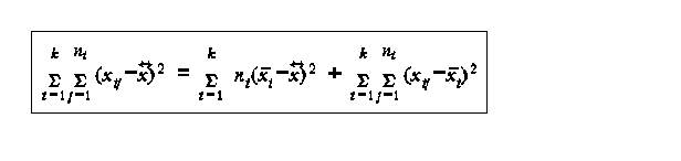
Total sum of squares = Between row sum of squares + within row sum of squares SST = SSR + SSE
where
Ti is the sum of all the observations in a row
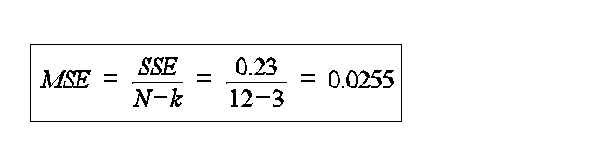
SSE=SST-SSR
SSE=.68 - .45 = 0.23
note the F ratio is slightly different when using the shortcut formula 8.823 vs 9.03 This a rare situation where the shortcut is actually a little less accurate than the long method
F distribution is One tail only (no such thing as a two tailed test), it doesn�t make sense to specify direction with k samples computed value of F (8.83) > critical value df1=2, df2=9, "=0.05, critical value=3.89 df1=2, df2=9, "=0.01, critical value=8.02 We can be > 99% certain the differences between the time periods are significant and that the observations in each time period are drawn from distributions with different population means
| |||||||||||||||||||||||||||||||||||||||||||||||||||||||||||||||||||||||||||||||||||||||||||||||||||||||||||||||||||||||||||||||||||||||||||||||||||||||||||||||||||||||||||||||||||||||||||||||||||||||||||||||||||||||||||||||||||||||||||||||
 T = sum of all
observations
T = sum of all
observations